7.2. Tutorial¶

In this tutorial, we explain through a sample calculation of the 8-site Hubbard model on the square lattice.

7.2.1. Run HPhi/vmc.out¶

For \({\mathcal H}\Phi\)

We calculate the ground state and the correlation function with the following input file

a0w = 2
a0l = 2
a1w = -2
a1l = 2
model="Hubbard"
method="CG"
lattice="square"
t=1.0
U=8.0
nelec = 8
2Sz=0

$ HPhi -s input

For mVMC

First, we optimize the trial wavefunction with the following input
```
a0w = 2
a0l = 2
a1w = -2
a1l = 2
model="Hubbard"
lattice="square"
t=1.0
U=8.0
nelec = 8
2Sz=0
```
```
$ vmc.out -s input
```
We add the following line to the input file to compute the correlation function.
```
NVMCCalMode = 1
```
Compute the correlation function.
```
$ vmc.out -s input output/zqp_opt.dat
```

Then the one- and two-body correlation function are written to files in the output/ directory.

Related files

StdFace.def (See the manuals for mVMC/\({\mathcal H}\Phi\))
zqp_opt.dat (See the manual for mVMC)
greenone.def (Specify the index of correlation function to be computed)
greentwo.def (Specify the index of correlation function to be computed)

7.2.2. Fourier transformation of correlation functions¶

Perform the Fourier transformation of the correlation function by using the utility greenr2k.

$ echo "4 20
G 0 0 0
X 0.5 0 0
M 0.5 0.5 0
G 0 0 0
16 16 1" >> geometry.dat
$ greenr2k namelist.def geometry.dat

Then the Fourier-transformed correlation functions are written to a file in output/.

Related files

output/zvo_cisajs_001.dat (Results of correlation function in the site representation)
output/zvo_cisajs.dat (Results of correlation function in the site representation)
output/zvo_cisajscktalt_001.dat (Results of correlation function in the site representation)
output/zvo_cisajscktalt.dat (Results of correlation function in the site representation)
geometry.dat (Geometry)
output/zvo_corr.dat (Correlation functions on the k path)

7.2.3. Display correlation functions¶

Plot the correlation function in the k space by using gnuplot.

load "kpath.gp"
plot "output/zvo_corr_eigen0.dat" u 1:12 w l

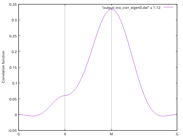
../_images/corplot.png — Fig. 7.1 The spin-spin correlation \(\langle{\bf S}_{\bf k}\cdot{\bf S}_{\bf k}\rangle\) (Column 12).¶

Related files

kpath.gp (gnuplot script)
output/zvo_corr.dat (Correlation functions on the k path)