4.1. Dynamical spin structure factor

Let’s solve the following Hubbard model on the square lattice.

(4.1)\[H = -t \sum_{\langle i,j\rangle , \sigma}(c_{i\sigma}^{\dagger}c_{j\sigma}+{\rm H.c.})+U \sum_{i} n_{i\uparrow}n_{i\downarrow}\]

The input files (samples/tutorial_4.1/stan1.in and samples/tutorial_4.1/stan2.in) for 8-site Hubbard model are as follows

stan1.in

a0W = 2
a0L = 2
a1W = -2
a1L = 2
model = "hubbard"
method = "CG"
lattice = "square"
t = 1.0
t' = 0.5
U = 4.0
2Sz = 0
nelec = 8
EigenvecIO = "out"

stan2.in

a0W = 2
a0L = 2
a1W = -2
a1L = 2
model = "hubbard"
method = "CG"
lattice = "square"
t = 1.0
t' = 0.5
U = 4.0
2Sz = 0
nelec = 8
LanczosEPS = 8
CalcSpec = "Normal"
SpectrumType = "SzSz"
SpectrumQW = 0.5
SpectrumQL = 0.5
OmegaMin = -10.0
OmegaMax = 20.0
OmegaIM = 0.2
OmegaOrg = 10.0

You can execute HPhi as follows

HPhi -s stan1.in
HPhi -s stan2.in

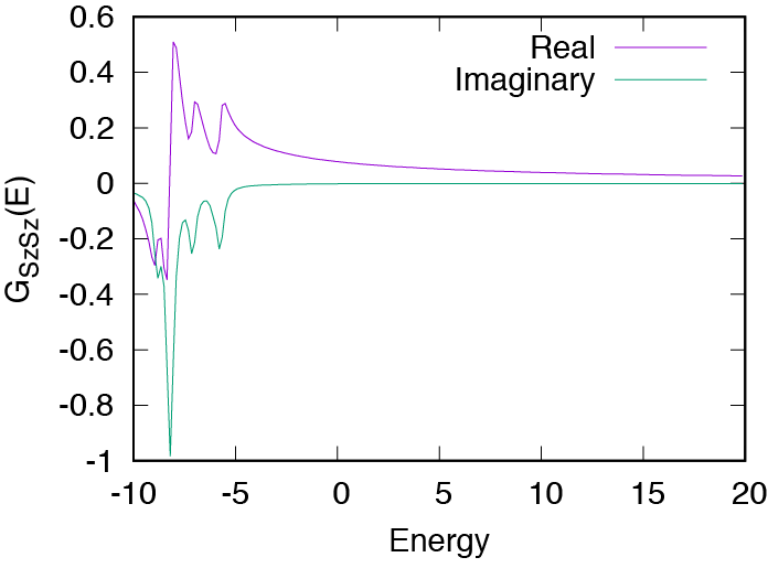
After finishing calculations, the spectrum \(G_{S_z S_z}({\bf Q} \equiv (\pi, \pi), \omega) = \langle S_z(-{\bf Q}) \left[H-\omega-\omega_0 + i\eta\right]^{-1}S_z({\bf Q})\rangle\) is outputted in output/zvo_DynamicalGreen.dat. Here, \(S_z({\bf Q})= \sum_{i}e^{i {\bf Q} \cdot {\bf r}_i} S_z^i\) and the frequency \(\omega\) moves from \(-10\) to \(10\), \(\omega_0 = 10\), and \(\eta\) is set as \(0.2\). You can check the result by executing the following command on gnuplot:

gnuplot
gnuplot> set xlabel "Energy"
gnuplot> set ylabel "G_{SzSz}(E)"
gnuplot> set xzeroaxis
gnuplot> plot "output/zvo_DynamicalGreen.dat" u 1:3 w l tit "Real", \
> "output/zvo_DynamicalGreen.dat" u 1:4 w l tit "Imaginary"

You can see the following output image.