Tutorial: How to Use Post-Processing Tools
Running PAMC Calculations
As an example, we’ll use a calculation from the TRHEPD forward problem solver (odatse-STR). The parameter space is 3-dimensional, with 51 temperature points logarithmically spaced from T=1.0 to 1.0e-6. Each annealing step consists of 20 MCMC steps. The number of replicas is set to 100 per process with 4 MPI processes.
Results are output under the output directory. MCMC calculation logs for each MPI process are written to output/{rank}/result_T{index}.txt, split by temperature points. The expected values and variances of f(x), along with partition function values, are output to output/fx.txt.
Note
If export_combined_files is set to True, logs are consolidated in combined.txt.
python3 extract_combined.py -t result.txt -d output
Run this to extract result.txt. Then split result.txt by temperature points.
extract_combined.py is a tool for extracting lines starting with specific tags, with the following options:
-t, --tag: Target tag for extraction (required)-d, --data_dir: Directory containing data files
For details, see extract_combined.py.
Note
If separate_T is False, logs are output to result.txt.
python3 separateT.py -d output
Run this to split into result_T{index}.txt files by temperature point.
separateT.py is a tool for splitting MCMC data files by temperature, with the following options:
-d, --data_dir: Directory containing data files-t, --file_type: Specific filename to split (processes result.txt in each directory if not specified)
For details, see separateT.py.
Calculating Model Evidence
The model evidence \(\log P(D;\beta)\) is expressed as:
\[\log P(D;\beta) = \log\left(\dfrac{Z_\beta}{Z_{\beta_0}}\right) - \log V_\Omega + \sum_\mu \dfrac{n_\mu}{2}\log\left(\dfrac{\beta w_\mu}{\pi}\right)\]Calculate model evidence using the partition function values \(\log Z/Z_0\) from output/fx.txt. This requires specifying the search space volume \(V_\Omega\) (normalization factor for prior probability) and the number of data points \(n\).
In this example, the search space spans [3.0, 6.0] for each of z1, z2, z3. The number of data points (rows in experiment.txt) is 70.
python3 plt_model_evidence.py -V 27.0 -n 70 output/fx.txt
Model evidence values are written to model_evidence.txt, and a plot against beta is output to model_evidence.png.
plt_model_evidence.py accepts these options:
-V, --Volume: Search space volume \(V_\Omega\)-n, --ndata: Number of data points (required)-o, --output: Output plot filename. The output format is determined by the file extension.
For details, see plt_model_evidence.py.
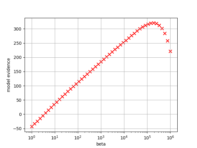
Fig. 13 Plot of model evidence. Maximum value occurs at beta= \(1.91\times 10^5\) (Tstep=44).
Summarizing Search Data by Temperature Points
Extract and combine replica configurations at the end of annealing from MCMC step information in output/{rank}/result_T{index}.txt.
python3 summarize_each_T.py -d output -o summarized
Results are written to summarized/result_T{index}_summarized.txt.
summarize_each_T.py extracts and combines replica configuration data for each temperature point, with these options:
-d, --data_directory: Directory containing MCMC data files-o, --export_directory: Output directory
Using the
-i, --input_fileoption with the TOML configuration file from the PAMC calculation automatically retrieves parameters such as the number of replicas.For details, see summarize_each_T.py.
Creating 1D and 2D Marginalized Histograms
Plot weighted posterior probability distributions \(P(z_i|D;\beta) = \dfrac{P(D|z_i\beta) P(z_i)}{P(D;\beta)}\) using replica configuration data.
To create 1D histograms marginalized along each \(z_i\):
python3 plt_1D_histogram.py -d summarized -o 1dhist -r 3.0,6.0
This creates histograms for each data file in summarized/, outputting to 1dhist/ as 1Dhistogram_result_T{index}_beta_{beta}.png (when the temperature range has been specified by bmin and bmax in the PAMC calculation), or 1Dhistogram_result_T{index}_T_{T}.png (when the temperature range has been specified by Tmin and Tmax in the PAMC calculation). Value range is set to 3.0-6.0.
plt_1D_histogram.py accepts these main options:
-d, --data_dir: Directory containing data files-o, --output_dir: Output directory-r, --range: Variable range (“min,max” format)-b, --bins: Number of histogram bins (default: 60)-f, --format: Output file formats (comma-separated list, default: “png”)--config: Configuration file path (TOML format)--params: Path to parameter file used in PAMC calculation
Using a configuration file allows setting multiple options together.
For details, see plt_1D_histogram.py.
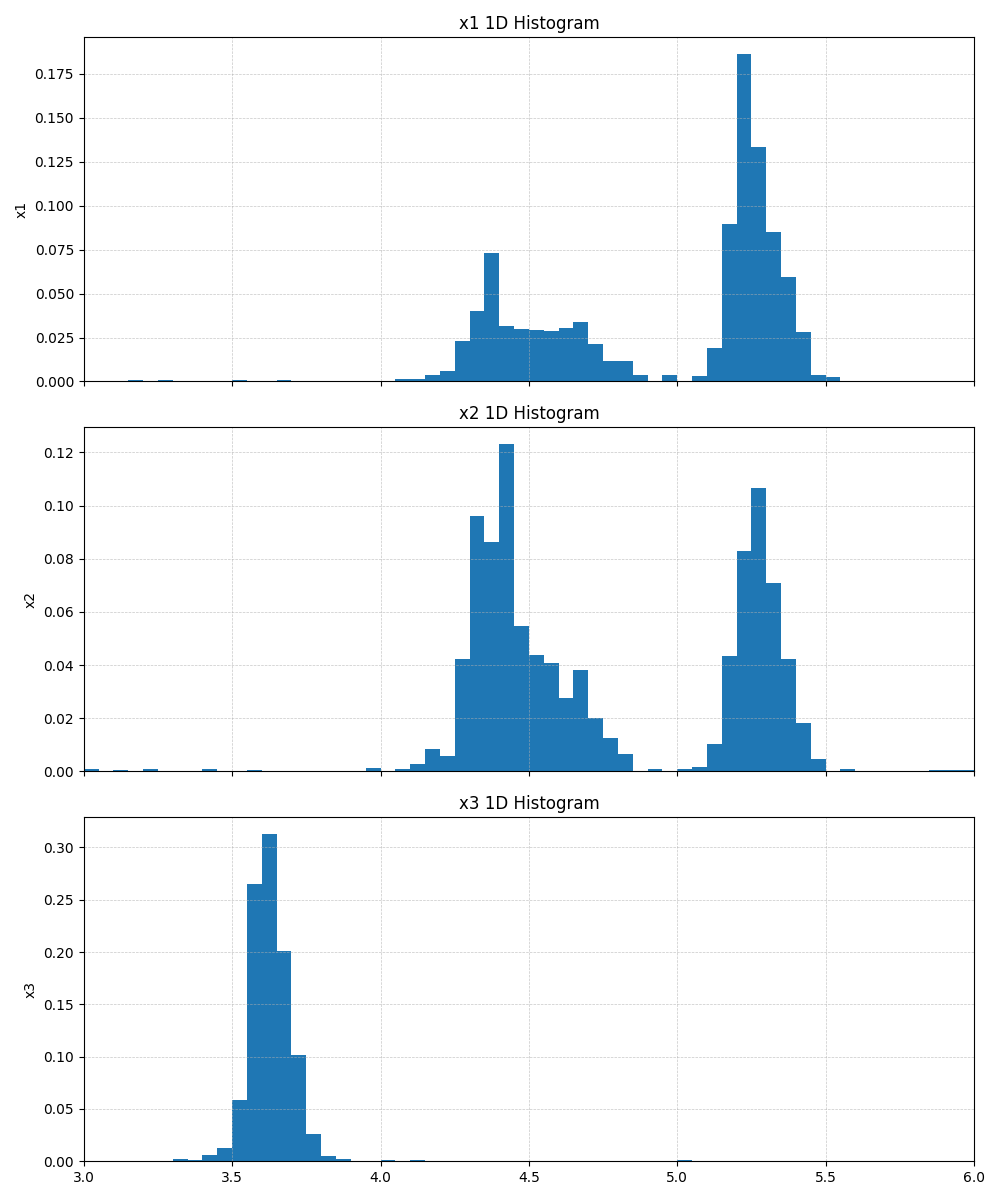
Fig. 14 Example 1D marginalized histogram output (Tstep=22, \(\beta=4.365\times 10^2\)).
To create 2D marginalized histograms:
python3 plt_2D_histogram.py -d summarized -o 2dhist -r 3.0,6.0
This creates 2D histograms for combinations (z1,z2), (z1,z3), (z2,z3), outputting to 2dhist/ as 2Dhistogram_result_T{index}_beta_{beta}_x1_vs_x2.png etc. (Axis labels are x1, x2, … if field_list not specified.)
plt_2D_histogram.py has the same options as plt_1D_histogram.py plus these features:
Generates histograms for each pair of variables
Visualizes probability density using logarithmic color mapping
Output filenames follow the pattern: 2Dhistogram_[filename]_[x-axis label]_vs_[y-axis label].[format]
Example: 2Dhistogram_result_T44_beta_1.91e+05_x1_vs_x2.png
For details, see plt_2D_histogram.py.
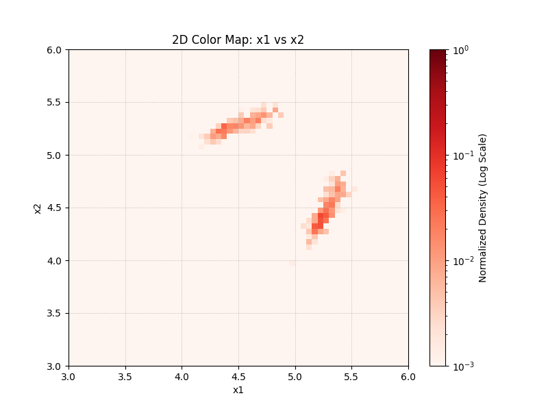
Fig. 15 Example 2D marginalized histogram output (Tstep=22, z1-z2 axis plot).