5.2. Input file for tenes_simple

• File format is TOML format.

• The input file has four sections : model, parameter, lattice, correlation .

  • The parameter section is copied to the standard mode input.

5.2.1. model section

Specify the model to calculate. In this version, spin system ("spin"), bosonic system ("boson"), spinless fermions ("spinless fermion"), and the fermionic Hubbard model ("hubbard") are defined.

Name	Description	Type	Default
type	Model type ("spin" / "boson" / "spinless fermion" / "hubbard")	String	–

The parameter names such as interactions depend on the model type.

Spin system: "spin"

Hamiltonian is described as

\[\mathcal{H} = \sum_{\langle ij \rangle}\left[\sum_\alpha^{x,y,z} J^\alpha_{ij} S^\alpha_i S^\alpha_j + B \left(\vec{S}_i\cdot\vec{S}_j\right)^2 \right] - \sum_i \sum_\alpha^{x,y,z} h^\alpha S^\alpha_i - \sum_i D \left(S^z_i\right)^2\]

The parameters of the one-body terms are defined as follows.

Name	Description	Type	Default
S	Magnitude of the local spin	Real (integer or half integer)	0.5
hx	Magnetic field along \(S^x\), \(h^x\)	Real	0.0
hy	Magnetic field along \(S^y\), \(h^y\)	Real	0.0
hz	Magnetic field along \(S^z\), \(h^z\)	Real	0.0
D	On-site spin anisotropy \(D\)	Real	0.0

The exchange interaction \(J\) can have a bond dependency.

Name	Description	Type	Default
J0	Exchange interaction of 0th direction nearest neighbor bond	Real	0.0
J1	Exchange interaction of 1st direction nearest neighbor bond	Real	0.0
J2	Exchange interaction of 2nd direction nearest neighbor bond	Real	0.0
J0'	Exchange interaction of 0th direction next nearest neighbor bond	Real	0.0
J1'	Exchange interaction of 1st direction next nearest neighbor bond	Real	0.0
J2'	Exchange interaction of 2nd direction next nearest neighbor bond	Real	0.0
J0''	Exchange interaction of 0th direction third nearest neighbor bond	Real	0.0
J1''	Exchange interaction of 1st direction third nearest neighbor bond	Real	0.0
J2''	Exchange interaction of 2nd direction third nearest neighbor bond	Real	0.0

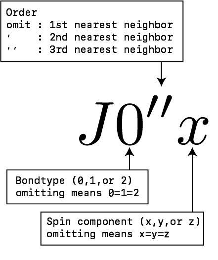
For the next nearest and third nearest neighbor bond, please surround the keyname with the double-quotation marks, ". The bond direction depends on the lattice defined in the lattice section. For a square lattice, for example, coupling constants along two bond directions can be defined, x-direction (0) and y-direction (1). By omitting the direction number, you can specify all directions at once. You can also specify Ising-like interaction by adding one character of xyz at the end. If the same bond or component is specified twice or more, an error will occur.

To summarize,

The biquadratic interaction \(B\) can also have a bond dependency like as \(J\).

Name	Description	Type	Default
B0	Biquadratic interaction of 0th direction nearest neighbor bond	Real	0.0
B1	Biquadratic interaction of 1st direction nearest neighbor bond	Real	0.0
B2	Biquadratic interaction of 2nd direction nearest neighbor bond	Real	0.0
B0'	Biquadratic interaction of 0th direction next nearest neighbor bond	Real	0.0
B1'	Biquadratic interaction of 1st direction next nearest neighbor bond	Real	0.0
B2'	Biquadratic interaction of 2nd direction next nearest neighbor bond	Real	0.0
B0''	Biquadratic interaction of 0th direction third nearest neighbor bond	Real	0.0
B1''	Biquadratic interaction of 1st direction third nearest neighbor bond	Real	0.0
B2''	Biquadratic interaction of 2nd direction third nearest neighbor bond	Real	0.0

One-site operators \(S ^ z\) and \(S ^ x\) are automatically defined. If parameter.general.is_real = false, \(S ^ y\) is also defined. In addition, bond Hamiltonian

\[\mathcal{H}_{ij} = \left[\sum_\alpha^{x,y,z} J^\alpha_{ij} S^\alpha_i S^\alpha_j + B \left(\vec{S}_i\cdot\vec{S}_j\right)^2 \right] - \frac{1}{z} \left[ \sum_\alpha^{x,y,z} h^\alpha \left(S^\alpha_i + S^\alpha_j \right) + D \left(\left(S^z_i\right)^2 + \left(S^z_j\right)^2 \right) \right],\]

and spin correlations on nearest neighbor bonds \(S^\alpha_iS^\alpha_j\) ( \(\alpha=x,y,z\) ) are automatically defined as two-site operators. In the bond Hamiltonian, one body terms (\(h^\alpha\) and \(D\) term) appear only in the nearest neighbor bonds, and \(z\) is the number of the coordinate number.

Bosonic system: "boson"

Hamiltonian is described as

\[\mathcal{H} = \sum_{i<j}\left[ -t_{ij} \left(b^\dagger_i b_j + b^\dagger_j b_i \right) + V_{ij} n_i n_j \right] + \sum_i \left[U\frac{n_i(n_i-1)}{2} - \mu n_i\right],\]

where \(b^\dagger\) and \(b\) are the creation and the annihilation operators of a boson, and \(n = b^\dagger b\) is the number operator.

The parameters of the one-body terms are defined as follows.

Name	Description	Type	Default
nmax	Maximum number of particles on a site	Integer	1
U	Onsite repulsion	Real	0.0
mu	Chemical potential	Real	0.0

The hopping constant \(t\) and the offsite repulsion \(V\) can have a bond dependency. Use t' and v' for second-neighbor bonds, and t'' and v'' for third-neighbor bonds. The typed forms such as t0' and v1'' select a bond type within a neighbor shell.

Name	Description	Type	Default
t0	Hopping of 0th direction nearest neighbor bond	Real	0.0
t1	Hopping of 1st direction nearest neighbor bond	Real	0.0
t2	Hopping of 2nd direction nearest neighbor bond	Real	0.0
t0'	Hopping of 0th direction next nearest neighbor bond	Real	0.0
t1'	Hopping of 1st direction next nearest neighbor bond	Real	0.0
t2'	Hopping of 2nd direction next nearest neighbor bond	Real	0.0
t0''	Hopping of 0th direction third nearest neighbor bond	Real	0.0
t1''	Hopping of 1st direction third nearest neighbor bond	Real	0.0
t2''	Hopping of 2nd direction third nearest neighbor bond	Real	0.0
V0	Offsite repulsion of 0th direction nearest neighbor bond	Real	0.0
V1	Offsite repulsion of 1st direction nearest neighbor bond	Real	0.0
V2	Offsite repulsion of 2nd direction nearest neighbor bond	Real	0.0
V0'	Offsite repulsion of 0th direction next nearest neighbor bond	Real	0.0
V1'	Offsite repulsion of 1st direction next nearest neighbor bond	Real	0.0
V2'	Offsite repulsion of 2nd direction next nearest neighbor bond	Real	0.0
V0''	Offsite repulsion of 0th direction third nearest neighbor bond	Real	0.0
V1''	Offsite repulsion of 1st direction third nearest neighbor bond	Real	0.0
V2''	Offsite repulsion of 2nd direction third nearest neighbor bond	Real	0.0

The bond direction depends on the lattice defined in the lattice section. For a square lattice, for example, coupling constants along two bond directions can be defined, x-direction (0) and y-direction (1). By omitting the direction number, you can specify all directions at once.

One-site operators \(n\), \(b\), and \(b^\dagger\) are automatically defined. In addition, bond Hamiltonian

\[\mathcal{H}_{ij} = \left[ -t_{ij} \left(b^\dagger_i b_j + b^\dagger_j b_i \right) + V_{ij} n_i n_j \right] + \frac{1}{z} \left[\left(U\frac{n_i(n_i-1)}{2} - \mu n_i\right) + (i \leftrightarrow j)\right]\]

and short range correlations on nearest neighbor bonds \(n_i n_j\), \(b^\dagger_i b_j\), and \(b_i b^\dagger_j\) are automatically defined as two-site operators. In the bond Hamiltonian, one body terms (\(U\) and \(\mu\) term) appear only in the nearest neighbor bonds, and \(z\) is the number of the coordinate number.

Spinless fermions: "spinless fermion"

Hamiltonian is described as

\[\mathcal{H} = \sum_{i<j}\left[ -t_{ij} \left(c^\dagger_i c_j + c^\dagger_j c_i \right) + V_{ij} n_i n_j \right] - \sum_i \mu n_i,\]

where \(c^\dagger\) and \(c\) are the creation and annihilation operators of a fermion, and \(n = c^\dagger c\) is the number operator. The local Hilbert-space dimension physical_dim is 2, and the local basis is \(|0\rangle\), \(|1\rangle\).

The parameter of the one-body term is defined as follows.

Name	Description	Type	Default
mu	Chemical potential	Real	0.0

The hopping constant \(t\) and the offsite repulsion \(V\) can have a bond dependency. Use t' and v' for second-neighbor bonds, and t'' and v'' for third-neighbor bonds. The typed forms such as t0' and v1'' select a bond type within a neighbor shell.

Name	Description	Type	Default
t	Hopping of a nearest-neighbor bond	Real	0.0
v	Offsite repulsion of a nearest-neighbor bond	Real	0.0

The one-site operators are automatically defined with the following group numbers: 0: n, 1: cdag, and 2: c. The parity-odd operators cdag and c are available for ops-form two-site observables and correlation functions; their one-site expectation values are always output as zero. In addition, hopping and nn on nearest-neighbor bonds are automatically defined as two-site operators. tenes_simple itself emits only nearest-neighbor two-site observables. To measure longer-distance two-site observables, add [[observable.twosite]] entries to the generated std.toml before running tenes_std.

Fermionic Hubbard model: "hubbard"

Hamiltonian is described as

\[\mathcal{H} = \sum_{i<j}\left[ -t_{ij} \sum_{\sigma=\uparrow,\downarrow} \left(c^\dagger_{i\sigma} c_{j\sigma} + c^\dagger_{j\sigma} c_{i\sigma} \right) + V_{ij} n_i n_j \right] + \sum_i \left[U n_{i\uparrow} n_{i\downarrow} - \mu n_i - h S^z_i\right].\]

This is the fermionic Hubbard model. The Bose-Hubbard model remains type = "boson". The local Hilbert-space dimension physical_dim is 4, and the local basis is \(|0\rangle\), \(|\uparrow\rangle\), \(|\downarrow\rangle\), \(|\uparrow\downarrow\rangle\). The ordering convention is \(|\uparrow\downarrow\rangle = c^\dagger_\uparrow c^\dagger_\downarrow |0\rangle\).

The parameters of the one-body terms are defined as follows.

Name	Description	Type	Default
u	Onsite repulsion	Real	0.0
mu	Chemical potential	Real	0.0
h	Magnetic field along \(S^z\)	Real	0.0

The hopping constant \(t\) and the offsite repulsion \(V\) can have a bond dependency.

Name	Description	Type	Default
t	Hopping of a nearest-neighbor bond	Real	0.0
v	Offsite repulsion of a nearest-neighbor bond	Real	0.0

One-site operators are automatically defined with the following group numbers: 0: n, 1: n_up, 2: n_dn, 3: Sz, 4: doublon, 5: holon, 6: cdag_up, 7: c_up, 8: cdag_dn, and 9: c_dn. The parity-odd operators cdag_up, c_up, cdag_dn, and c_dn are available for ops-form two-site observables and correlation functions; their one-site expectation values are always output as zero. In addition, hopping, nn, SzSz, SxSx, and SySy on nearest-neighbor bonds are automatically defined as two-site operators. The spin operators are \(S^\alpha = \frac{1}{2}\sum_{ss'} c^\dagger_s \sigma^\alpha_{ss'} c_{s'}\). Two-site values in density.dat are per site (the sum over bonds divided by the number of sites with a physical dimension larger than 1, that is, excluding vacancies), so on the square lattice they are twice the correlation per nearest-neighbor bond. tenes_simple itself emits only nearest-neighbor two-site observables. To measure longer-distance two-site observables, add [[observable.twosite]] entries to the generated std.toml before running tenes_std.

Beyond-nearest-neighbor Hamiltonian bonds in fermion mode are supported with the simple update only; they are rejected when the full update has a positive num_step. See the lattice section for the fermionic lattices and neighbor ranges supported by tenes_simple. With the CTM environment, two-site observables are available in the 4 x 4 window (|dx| <= 3 and |dy| <= 3) and may use either explicit elements or ops = [A, B]. With meanfield_env = true, the same longer-distance two-site observables and correlation functions are available using the mean-field approximation, where the outside of the measured window is closed by the simple-update \(\lambda\) weights.

5.2.2. lattice section

Specify the lattices to calculate. Square, triangular, honeycomb, and Kagome lattices are defined.

Name	Description	Type	Default
type	lattice name (square, triangular, honeycomb or kagome lattice)	String	–
L	Unit cell size in x direction	Integer	–
W	Unit cell size in y direction	Integer	L
virtual_dim	Bond dimension	Integer	–
initial	Inital state	String	random
noise	Noise for elements in initial tensor	Real	1e-2

initial and noise are parameters that determine the initial state of the wave function. If tensor_load is set in parameter.general, initial is ignored.

• initial

  • "ferro" : Ferromagnetic state

    • In spin system, all sites has \(S^z = S\)

    • In bosonic system, all sites has \(n = n_{\text{max}}\) particles

  • "antiferro" : Antiferromagnetic state

    • In spin system, for square lattice and honeycomb lattice, the Neel order state (\(S^z = S\) for the A sublattice and \(S^z = -S\) for the B sublattice), and for triangular lattice and kagome lattice, the 120 degree order state (spins on sites belonging to the A, B, and C sublattice are pointing to \((\theta, \phi) = (0,0), (2\pi/3, 0)\) and \((2\pi/3, \pi)\) direction, respectively.)

    • In bosonic system, sites belonging to one sublattice have \(n_\text{max}\) particles and the other sites have no particles.

  • "random" : Random state

  • In fermionic models, "random" and "vacuum" are available for spinless fermions, and "random", "vacuum", "full", and "cdw" are available for the Hubbard model. "ferro" and "antiferro" are not available because product states containing odd-parity local states cannot be built.

• noise

  • The amount of fluctuation in the elements of the initial tensor

In fermionic models, tenes_simple supports Hamiltonian bonds up to third neighbors on square, triangular, honeycomb, and kagome lattices. On the kagome lattice, nearest-neighbor bonds in one direction are two-hop chains in the square-lattice embedding, so even a nearest-neighbor kagome model uses the long-range gate chain and is restricted to the simple update when those bonds are present.

Square lattice

A square lattice type = "square lattice" consists of L sites in the \((1,0)\) direction and W sites in the \((0,1)\) direction. As a concrete example, Fig. 5.1 (a) shows the structure for L=3, W=3. In addition, the definitions of the first, second and third nearest neighbor bonds are shown in Fig. 5.1 (b), (c), and (d), respectively. The blue line represents a bond of bondtype = 0 and the red line represents a bond of bondtype = 1.

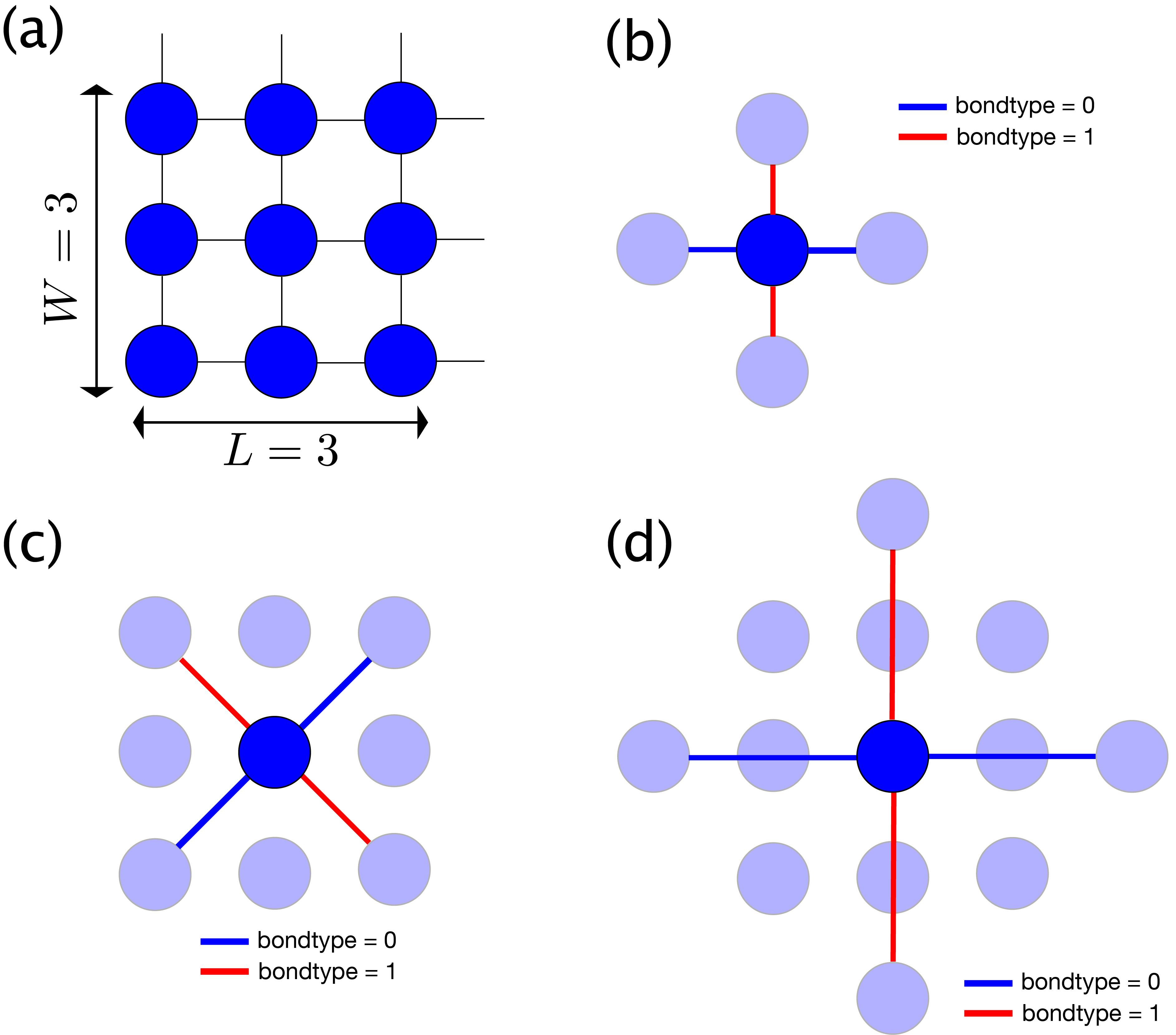
Fig. 5.1 Square lattice. (a) Site structure with L=3, W=3 (b) Nearest neighbor bonds. bondtype=0 (blue) bond extends in the 0 degree direction and bondtype=1 (red) one in the 90 degree direction. (c) Second nearest neighbor bonds. bondtype=0 (blue) bond extends in the 45 degree direction and bondtype=1 (red) one in the -45 degree direction. (d) Third nearest neighbor bonds. bondtype=0 (blue) bond extends in the 0 degree direction and bondtype=1 (red) one in the 90 degree direction.

Triangular lattice

A triangular lattice type = "triangular lattice" consists of L sites in the \((1,0)\) direction and W sites in the \((1/2, \sqrt{3}/2)\) direction. As a concrete example, Fig. 5.2 (a) shows the structure for L=3, W=3. In addition, the definitions of the first, second and third nearest neighbor bonds are shown in Fig. 5.2 (b), (c), and (d), respectively. The blue, red, and green lines represent bonds of bondtype = 0, 1, and 2, respectively. (e) shows the corresponding square TPS with L=3, W=3.

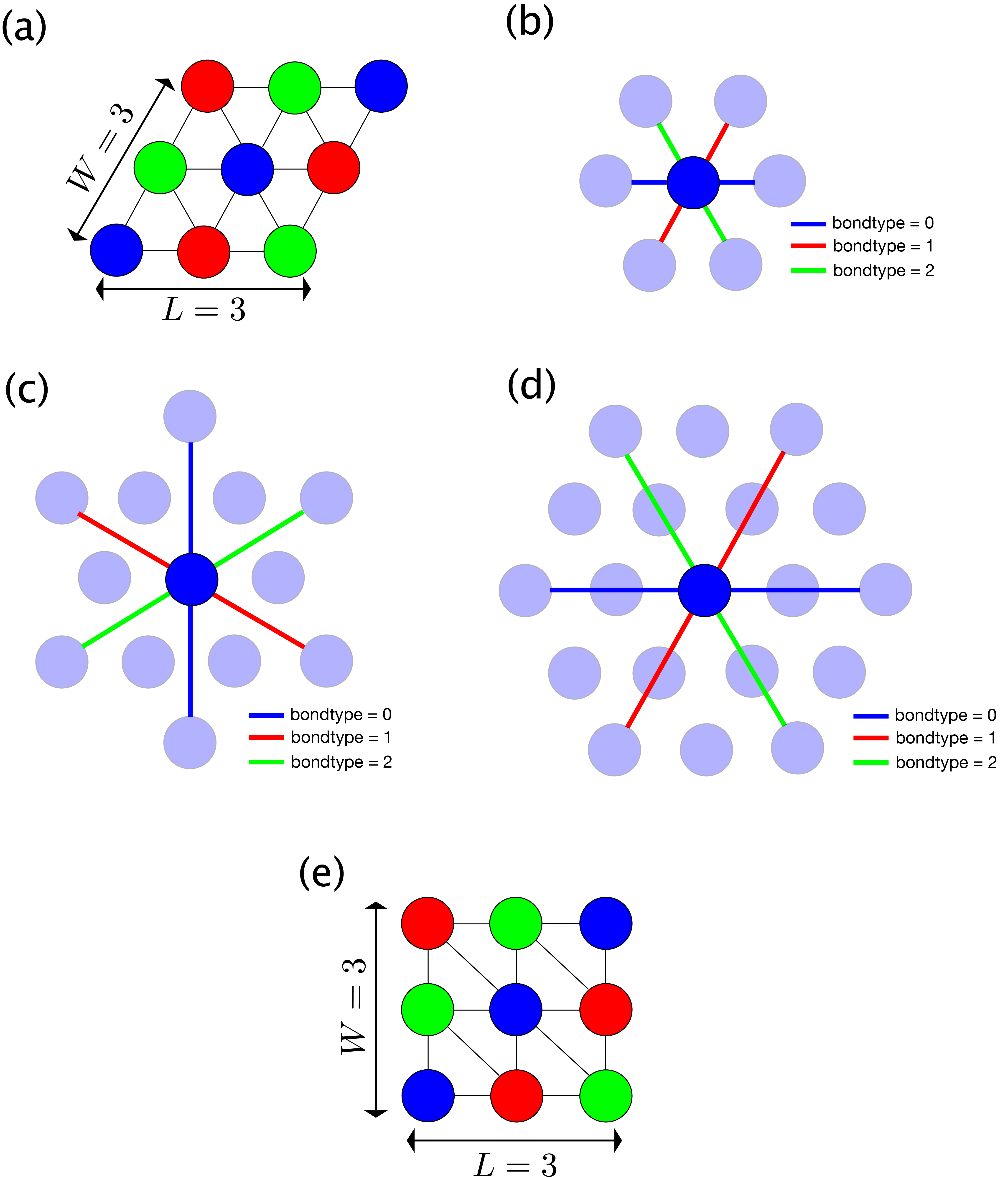
Fig. 5.2 Triangular lattice. (a) Site structure with L=3, W=3 (b) Nearest neighbor bonds. bondtype=0 (blue) bond extends in the 0 degree direction, bondtype=1 (red) one in the 60 degree direction, and bondtype=2 (green) one in the 120 degree direction. (c) Second nearest neighbor bonds. bondtype=0 (blue) bond extends in the 90 degree direction, bondtype=1 (red) one in the -30 degree direction, and bondtype=2 (green) one in the 30 degree direction. (d) Third nearest neighbor bonds. bondtype=0 (blue) bond extends in the 0 degree direction, bondtype=1 (red) one in the 60 degree direction, and bondtype=2 (green) one in the 120 degree direction. (e) Corrensponding square TPS of the triangular lattice with L=3, W=3.

Honeycomb lattice

In a honeycomb lattice type = "honeycomb lattice", units consisting of two sites of coordinates \((0, 0)\) and \((\sqrt{3}/2, 1/2)\) are arranged with L units in the \((\sqrt{3},0)\) direction and W units in the \((1/2, 3/2)\) direction. As a concrete example, Fig. 5.3 (a) shows the structure for L=2, W=2. In addition, the definitions of the first, second and third nearest neighbor bonds are shown in Fig. 5.3 (b), (c), and (d), respectively. The blue, red, and green lines represent bonds of bondtype = 0, 1, and 2, respectively. (e) shows the corresponding square TPS with L=2, W=2.

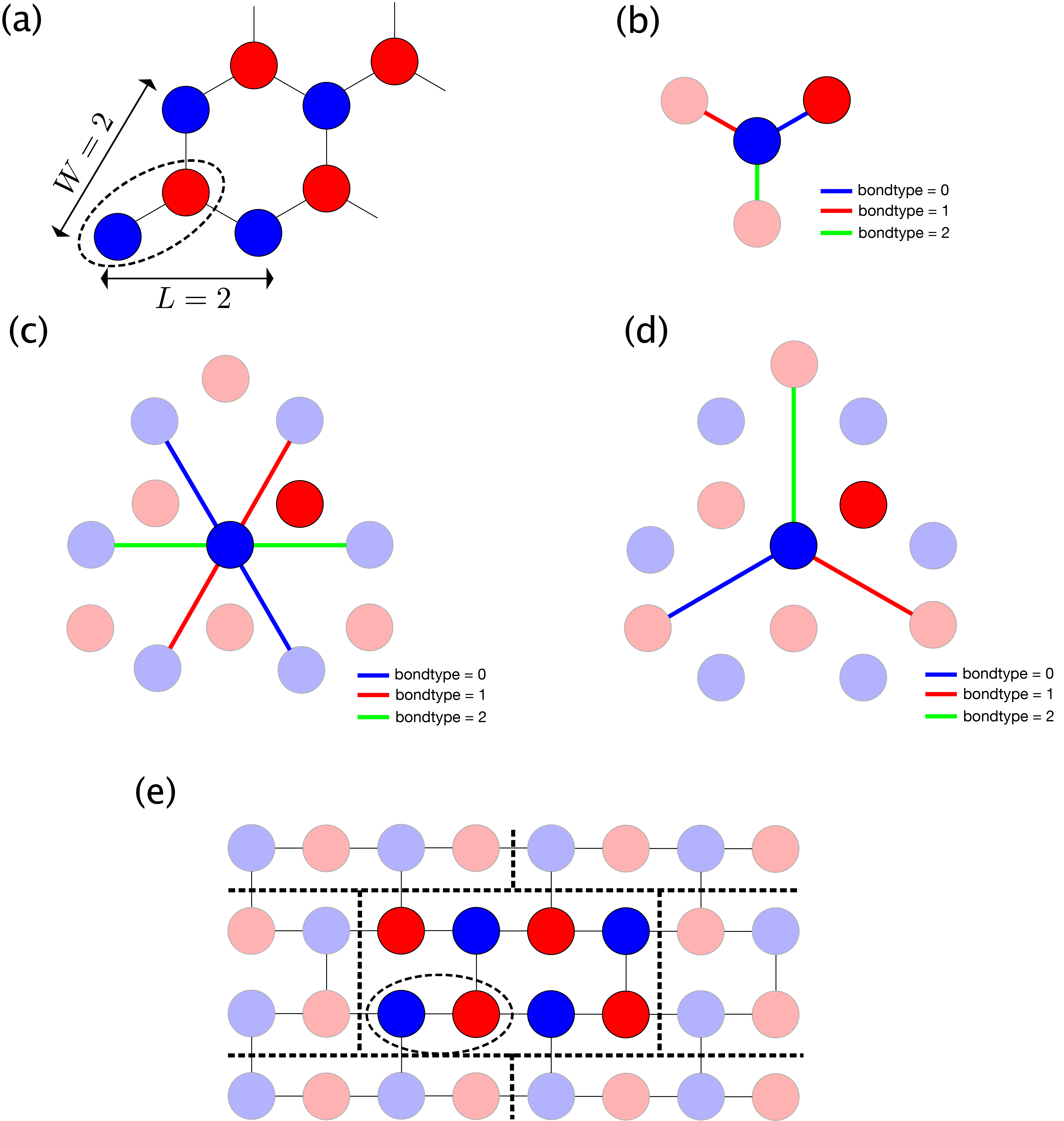
Fig. 5.3 Honeycomb lattice. (a) Site structure with L=2, W=2. The dashed ellipse denotes one unit. (b) Nearest neighbor bonds. bondtype=0 (blue) bond extends in the 30 degree direction, bondtype=1 (red) one in the 150 degree direction, and bondtype=2 (green) one in the -90 degree direction. (c) Second nearest neighbor bonds. bondtype=0 (blue) bond extends in the 120 degree direction, bondtype=1 (red) one in the 60 degree direction, and bondtype=2 (green) one in the 0 degree direction. (d) Third nearest neighbor bonds. bondtype=0 (blue) bond extends in the -30 degree direction, bondtype=1 (red) one in the -150 degree direction, and bondtype=2 (green) one in the 90 degree direction. (e) Corresponding square TPS of the honeycomb lattice with L=2, W=2. Note that the most top-right red tensor in the honeycomb lattice moves to the most top-left position, and the boundary condition is skewed.

Kagome lattice

In a kagome lattice type = "kagome lattice", units consisting of three sites of coordinates \((0, 0)\), \((1, 0)\), and \((1/2, \sqrt{3}/2)\) are arranged with L units in the \((2,0)\) direction and W units in the \((1,\sqrt{3})\) direction. As a concrete example, Fig. 5.4 (a) shows the structure for L=2, W=2. In addition, the definitions of the first, second and third nearest neighbor bonds are shown in Fig. 5.4 (b), (c), and (d), respectively. The blue and the red lines represent bonds of bondtype = 0, and 1, respectively. (e) shows the corresponding square TPS with L=2, W=2. In fermionic models, the dummy tensor in this square-lattice embedding is a vacancy with physical dimension 1 and even parity. tenes writes the energy in density.dat per site with a physical dimension larger than 1, so for the kagome lattice it is per non-vacancy site.

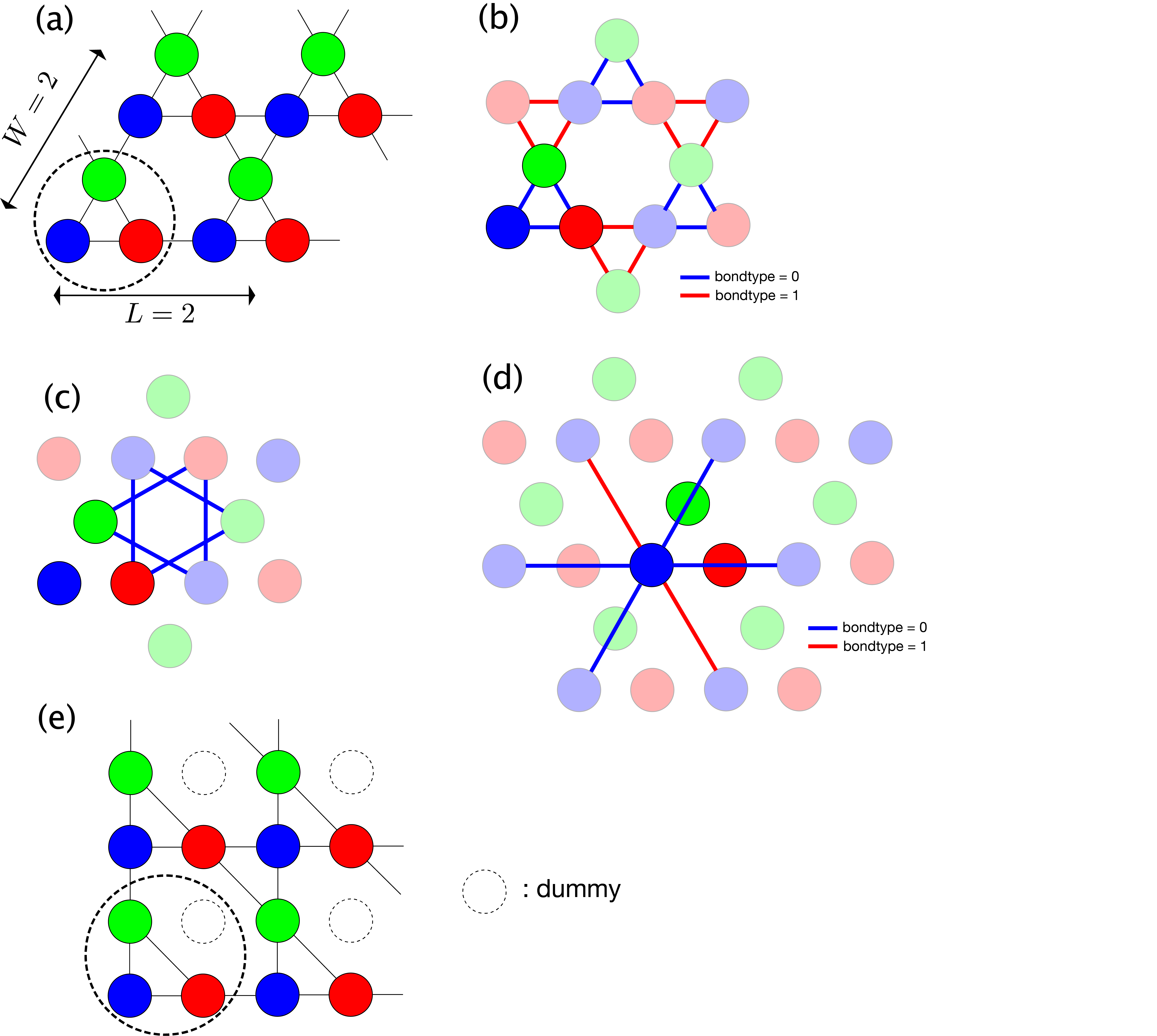
Fig. 5.4 Kagome lattice. (a) Site structure with L=2, W=2. The dashed circle denotes one unit. (b) Nearest neighbor bonds. bondtype=0 (blue) bonds form upper triangle and bondtype=1 (red) bonds form lowertriangle. (c) Second nearest neighbor bonds. (d) Third nearest neighbor bonds. bondtype=0 (blue) bond passes over a site and bondtype=1 (red) one does not. (e) Corresponding square TPS of the kagome lattice with L=2, W=2. The white circles are the dummy tensors with bonds of dimension one.

5.2.3. parameter section

Parameters defined in this section is not used in tenes_simple but they are copied to the input file of tenes_std.

Set various parameters that appear in the calculation, such as the number of updates. This section has five subsections: general, simple_update, full_update, ctm, random.

parameter.general

General parameters for tenes.

Name	Description	Type	Default
mode	Calculation mode	String	\"ground state\"
is_real	Whether to limit all tensors to real valued ones	Boolean	false
fermion	Whether the model is fermionic (experimental)	Boolean	false
iszero_tol	Absolute cutoff value for reading operators	Real	0.0
measure	Whether to calculate and save observables	Boolean	true
measure_interval	Interval of measurement in finite temperature calculation and time evolution process	Integer or list of integers	10
output	Directory for saving result such as physical quantities	String	"output"
tensor_save	Directory for saving optimized tensors	String	""
tensor_load	Directory for loading initial tensors	String	""

• mode

  • Specify the calculation mode

  • "ground state"

    • Search for the ground state of the Hamiltonian

    • tenes_std calculates the imaginary time evolution operator \(U(\tau) = e^{-\tau H}\) from the Hamiltonian \(H\)

  • "time evolution"

    • Calculate the time evolution of the observables from the initial state

    • tenes_std calculates the time evolution operator \(U(t) = e^{-it H}\) from the Hamiltonian \(H\)

  • "finite temperature"

    • Calculate the finite temperature expectation values of the observables

    • tenes_std calculates the imaginary time evolution operator \(U(\tau) = e^{-\tau H}\) from the Hamiltonian \(H\)

• is_real

  • When set to true, the type of elements of the tensor becomes real.

  • If one complex operator is defined at least, calculation will end in errors before starting.

• fermion

  • Experimental. When set to true, site tensors are treated as fermionic (Z2-graded) tensors and all bond updates and measurements generate the fermionic exchange signs automatically

  • The implementation follows the Z2-graded (super vector space) formulation of fermionic tensor networks: every leg carries a parity, and transpositions, contractions and decompositions generate the exchange signs. For the formulation, see Q. Mortier et al., SciPost Phys. 18, 012 (2025); N. Bultinck, D. J. Williamson, J. Haegeman, and F. Verstraete, Phys. Rev. B 95, 075108 (2017); N. Bultinck, D. J. Williamson, J. Haegeman, and F. Verstraete, J. Phys. A: Math. Theor. 51, 025202 (2018). Where the bra and ket layers cross in a measurement, the signs are the swap gates of the equivalent formulation by P. Corboz, R. Orús, B. Bauer, and G. Vidal, Phys. Rev. B 81, 165104 (2010)

  • Each site must declare the parity of its physical basis states by the parity key of the tensor.unitcell section, defined with respect to a fixed internal ordering of the creation operators on the site (see the tensor.unitcell section)

  • Operator and gate matrix elements: the elements of a two-site operator (elements with indices i1 i2 o1 o2) are the matrix elements \(\langle o_1 o_2 | O | i_1 i_2 \rangle\) in the ordered two-site Fock basis

    \[|i_1 i_2\rangle = A^\dagger_1(i_1)\, A^\dagger_2(i_2)\, |0\rangle\]

    where \(A^\dagger(i)\) is the creation-operator string of the local basis state \(i\) in the fixed internal order, and site 1 is source_site. These matrix elements must be evaluated with the fermionic anticommutation relations.

    • Example: for spinful electrons, \(\langle \uparrow\downarrow, 0 |\, c^\dagger_{1\uparrow} c_{2\uparrow} \,| \downarrow, \uparrow \rangle = -1\). Rather than writing the signs by hand, build the two-site Fock space of the modes involved numerically (Jordan-Wigner) and read the matrix elements off

    \[\langle \uparrow\downarrow, 0 |\, c^\dagger_{1\uparrow} c_{2\uparrow} \,| \downarrow, \uparrow \rangle = \langle 0 |\, c_{1\downarrow} c_{1\uparrow} c^\dagger_{1\uparrow} c_{2\uparrow} c^\dagger_{1\downarrow} c^\dagger_{2\uparrow} \,| 0 \rangle = \langle 0 |\, c_{1\downarrow} c_{1\uparrow} c^\dagger_{1\uparrow} \left(- c^\dagger_{1\downarrow} c_{2\uparrow}\right) c^\dagger_{2\uparrow} \,| 0 \rangle = -1\]

  • All exchange signs between sites (including those from the two-dimensional geometry) are generated by TeNeS; the user supplies only the correctly signed local matrices above

  • Evolution gates and two-site operators must conserve fermion parity. A one-site observable may be parity odd, but its one-site expectation value is then exactly zero; parity-odd one-site operators are useful as factors in ops-form two-site observables and in [correlation]

    • For instance, the expectation value of a single creation or annihilation operator is reported as zero.

  • In the current version fermion mode supports the ground-state calculation and the time evolution (mode = "time evolution") with the simple update (CTM or mean-field environment) and the full update (CTM environment only). Two-site observables may use explicit elements or ops = [A, B] and may be measured in the 4 x 4 window (|dx| <= 3 and |dy| <= 3); [correlation] is also available and writes \(\langle A_s B_t\rangle\), with \(A\) on the left or lower site. Operator pairs with different fermion parity are output as zero. With meanfield_env = true, longer-distance two-site observables and correlation functions are evaluated by closing the outside of the measured window or chain with the simple-update \(\lambda\) weights. Beyond-nearest-neighbor Hamiltonian bonds are supported in fermion mode with the simple update; the full update rejects such bonds when full_update.num_step > 0. Hamiltonian bonds outside the 4 x 4 window are rejected because their energy cannot be measured in fermion mode. Use_RSVD, Simple_Gauge_Fix, finite temperature, multi-site observables, and unit cells in which a site is its own nearest neighbor (LX = 1, or LY = 1 with skew = 0) are not available and are rejected when the input is read. The correlation length is likewise unavailable: tenes_simple rejects a [correlation_length] table for a fermionic model, and the solver disables the measurement with a warning at the point of measurement

  • The time evolution in fermion mode starts from a product state of even-parity sites (such as the vacuum, or doubly occupied and empty sites), from a random even-parity state, or from a state loaded by tensor_load (e.g., a ground state, for a quench). A product state with an odd-parity site is rejected, as in the ground-state calculation. Starting the full update directly from a product state with a large bond dimension (e.g., D = 8) can stop at the parity projection of the first steps, because most of the virtual space is still empty; start with a smaller D, or use the simple update.

  • With beyond-nearest-neighbor Hamiltonian bonds at small bond dimension, such as D = 2, a random initial state can fall into the vacuum and stay there. Start from a state converged with nearest-neighbor terms only by using tensor_save and tensor_load, or use a larger D.

  • In fermion mode, a two-site gate with an output index that has no nonzero element is rejected when the input is read, even for a nearest-neighbor bond. Non-invertible gates such as projectors can have this form; gates of the form \(\exp(-\tau h)\) are not affected.

• iszero_tol

  • When the absolute value of operator elements loaded is less than iszero_tol, it is regarded as zero

• meaure

  • When set to false, the stages for measuring and saving observables will be skipped

  • Elapsed time time.dat is always saved

• measure_interval

  • Specify the interval of measurement in time evolution process and finite temperature Calculation

  • Physical quantitites are calculated and saved each after measure_interval updates

• output

  • Save numerical results such as physical quantities to files in this directory

  • Empty means "." (current directory)

• tensor_save

  • Save optimized tensors to files in this directory

  • If empty no tensors will be saved

  • See Checkpoint files below for how a checkpoint is saved and what to do when a save was interrupted

• tensor_load

  • Read initial tensors from files in this directory

  • If empty no tensors will be loaded

  • It may be the same directory as tensor_save. See Checkpoint files below

Checkpoint files (tensor_save and tensor_load)

A run saves its tensors into the tensor_save directory as a checkpoint, and a later run reads it back from tensor_load. Both may name the same directory, so that each run continues from the previous run’s checkpoint and replaces it.

• Saving

  • A checkpoint is built in a working directory <destination>/.tenes-save-tmp/ and moved into place one file at a time once it is complete. A run killed while writing therefore leaves the previous checkpoint in the destination, intact. The working directory is removed when the save finishes, and one left by a run that died is removed by the next save

  • The working directory and the checkpoint exist side by side just before the move, so the disk usage during a save peaks at twice the size of a checkpoint

  • Checkpoint files that the save does not write are removed from the destination, so saving over a checkpoint of a calculation with more sites or more MPI processes leaves none of the earlier run’s files behind. Files that are not part of a checkpoint are left alone

  • Do not point two concurrent runs at the same tensor_save directory: each would overwrite the other’s working directory

  • If the checkpoint cannot be written, ``tenes`` exits with a non-zero status, after writing its measurement files as usual. Every file of the checkpoint is checked once it is written, including the tensor data each MPI process writes, so a file cut short by a full disk or a quota counts as a failure. Discarding a finished computation over a failed save would be worse, but an exit status of 0 would let a chain such as tenes A && tenes B, where B reloads A’s checkpoint, silently restart from a stale one. An error the file system reports only later, or damage done to the files after the save, is not detected

• When a save was interrupted while moving its files

  • If a run dies, or a file cannot be moved, while the checkpoint is being moved into place, <destination>/.tenes-save-incomplete is left behind. The destination may then hold a mixture of the new checkpoint and the previous one, so tensor_load refuses it and shows what that file says

  • To repair it by hand, move everything that is left in <destination>/.tenes-save-tmp/ into the destination, then delete .tenes-save-incomplete. That file gives the same instructions together with the full path of the working directory

  • A later save into the same destination does that repair itself before writing anything. If a file cannot be moved then either, it stops at that file, saves nothing, and exits with a non-zero status. The files not moved yet are still in the working directory and .tenes-save-incomplete is still there, so the repair by hand above still applies

  • If only .tenes-save-incomplete itself cannot be deleted, at the end of a save or after that repair, tenes says so and exits with a non-zero status. Every file is in place then, and deleting that file by hand is all that is left

• Loading

  • A checkpoint is refused, on every MPI process, when its number of sites differs from the input, or when one of the checkpoint and the input is fermionic and the other is not

  • Tensors saved by a real-valued calculation (is_real = true) can be loaded into a complex-valued one, such as a time evolution started from a ground state; they are converted on loading. Tensors saved by a complex-valued calculation cannot be loaded into a calculation with is_real = true, and the load is refused. A tensor file whose header records no element type (value_type), which no released TeNeS writes, is refused as well

  • The bond dimension may be changed from that of the saved tensors. Enlarging pads the new components with zeros and shrinking simply truncates. In a fermionic system, however, shrinking is not available in the current version, because the parity ledger of the virtual bonds has to be truncated consistently.

  • When the bond dimension is enlarged, the added components are zero, so a simple update or a full update has to be run after loading before the enlarged space is actually used. Measurement alone will not populate it.

parameter.simple_update

Parameters in the simple update procedure.

Name	Description	Type	Default
tau	(Imaginary) time step \(\tau\) in (imaginary) time evolution operator	Real or list of real	0.01
num_step	Number of simple updates	Integer or list of integers	0
lambda_cutoff	cutoff of the mean field to be considered zero in the simple update	Real	1e-12
gauge_fix	Whether the tensor gauge is fixed	Boolean	false
gauge_maxiter	Maximum number of iterations for fixing gauge	Integer	100
gauge_converge_epsilon	Convergence criteria of iterations for fixing gauge	Real	1e-2

• tau

  • Specify the (imaginary) time step \(\tau\) in (imaginary) time evolution operator

    • tenes_std uses it to calculate the imaginary time evolution operator \(e^{-\tau H}\) from the Hamiltonian

    • tenes uses it to calculate the time of each measurement

      • For finite temperature calculation, note that the inverse temperature increase \(2\tau\) at a step because \(\rho(\beta + 2\tau) = U(\tau)\rho(\beta)\bar{U}(\tau)\)

  • When a list is specified, the time step can be changed for each group of time evolution operators

• num_step

  • Specify the number of simple updates

  • When a list is specified, the number of simple updates can be changed for each group of time evolution operators

parameter.full_update

Parameters in the full update procedure.

Name	Description	Type	Default
tau	(Imaginary) time step \(\tau\) in (imaginary) time evolution operator	Real or list of reals	0.01
num_step	Number of full updates	Integer or list of integers	0
env_cutoff	Cutoff of singular values to be considered as zero when computing environment through full updates	Real	1e-12
inverse_precision	Cutoff of singular values to be considered as zero when computing the pseudoinverse matrix with full update	Real	1e-12
convergence_epsilon	Convergence criteria for truncation optimization with full update	Real	1e-6
iteration_max	Maximum iteration number for truncation optimization on full updates	Integer	100
gauge_fix	Whether the tensor gauge is fixed	Boolean	true
fastfullupdate	Whether the fast full update is adopted	Boolean	true

• Notes

  • The full update supports only the CTM environment, and combining it with meanfield_env = true is an error

  • The plain path (fastfullupdate = false) reconverges the CTM after every bond and is slower than the fast full update (about 9 times for free fermions at D = 3, chi = 12). In a fermionic system this reconvergence starts from the environment of the previous bond (a warm start); the bosonic plain path still converges from uniform vectors every time

  • If a full update stops at the forbidden-parity guard, the CTM has not converged, typically because dimension (chi) is too small for the state (the CTM then keeps cycling instead of settling). Increase dimension of [parameter.ctm] first, then iteration_max, and run the simple update longer if the state itself is far from converged

  • The two-site environment of the full update has to conserve fermion parity. If the violation (typically caused by an unconverged CTM) exceeds the threshold, which is the larger of 1e-8 and 100 times convergence_epsilon of [parameter.ctm], the run stops with an error; increase iteration_max or decrease convergence_epsilon in [parameter.ctm] in that case

  • For small bond dimensions (e.g. D = 2 for free fermions) the full update started from a converged simple-update state can raise the energy. This is because the fixed point of the projected imaginary-time evolution can lie above the simple-update fixed point when the variational space is too small.

parameter.ctm

Parameters for corner transfer matrices, CTM.

Name	Description	Type	Default
dimension	Bond Dimension of CTM \(\chi\)	Integer	4
projector_cutoff	Cutoff of singular values to be considered as zero when computing CTM projectors	Real	1e-12
convergence_epsilon	CTM convergence criteria	Real	1e-6
use_onesite_rdm_convergence	Use one-site RDM distances between CTM iterations for convergence	Boolean	true
iteration_max	Maximum iteration number of convergence for CTM	Integer	100
projector_corner	Whether to use only the 1/4 corner tensor in the CTM projector calculation	Boolean	true
use_rsvd	Whether to replace SVD with random SVD	Boolean	false
rsvd_oversampling_factor	Ratio of the number of the oversampled elements to that of the obtained elements in random SVD method	Real	2.0
meanfield_env	Use mean field environment obtained through simple update instead of CTM. Also available in fermion mode, where observables and correlations close the outside of the measured window or chain with simple-update lambda weights (much cheaper than the CTM path, with simple-update-level accuracy)	Boolean	false

When use_onesite_rdm_convergence is true, CTM convergence is checked by using the singular-value spectrum of the corner transfer matrices and the distance between one-site reduced density matrices in successive iterations. The distance is the maximum elementwise norm over all sites and matrix elements, divided by the trace of the density matrix, so that it contains both the change of the shape of the density matrix and the relative change of its norm. This avoids false convergence detected only from the corner spectrum on a network that virtual bonds of dimension one decompose into independent pieces, for example a quasi-one-dimensional calculation where the horizontal virtual bond dimension is set to one (see also the description of the algorithm). (Note that this is not a recommendation to run such a quasi-one-dimensional calculation; TeNeS targets two-dimensional lattices.) When it is false, TeNeS uses the previous criterion based only on the corner spectrum. The residual error of observables at convergence is typically on the scale of convergence_epsilon; decrease convergence_epsilon when higher accuracy is required.

For Tensor renomalization group approach using random SVD, please see the following reference, S. Morita, R. Igarashi, H.-H. Zhao, and N. Kawashima, Phys. Rev. E 97, 033310 (2018) .

parameter.random

Parameters for random number generators.

Name	Description	Type	Default
seed	Seed of the pseudo-random number generator used to initialize the tensor	Integer	11

Each MPI process has the own seed as seed plus the process ID (MPI rank).

Example

[parameter]
[parameter.general]
is_real = true
[parameter.simple_update]
num_step = 100
tau = 0.01
[parameter.full_update]
num_step = 0  # No full update
tau = 0.01
[parameter.ctm]
iteration_max = 10
dimension = 9 # CHI

5.2.4. correlation section

For tenes_simple , correlation functions \(C = \langle A(0)B(r)\rangle\) are not calculated by default. For calculating correlation functions, they have to be specified in the same file format as the input file of tenes. For fermionic spinless models, omitting operators selects [[0, 0], [1, 2]]; for fermionic Hubbard models it selects [[0, 0], [1, 1], [2, 2], [3, 3], [4, 4], [5, 5], [6, 7], [8, 9]]. Fermionic correlation functions are available with the CTM environment and with meanfield_env = true; in the mean-field case the outside of the correlation chain is closed approximately with the simple-update \(\lambda\) weights. Pairs with different operator parity are output as zero. For details, See correlation section Input file for tenes.

5.2.5. correlation_length section

Parameters defined in this section is not used in tenes_simple but they are copied to the input file of tenes_std.

This section describes how to calculate the correlation length \(\xi\).

Name	Description	Type	Default
measure	Whether to calculate \(xi\) or not	Bool	true
num_eigvals	The number of eigenvalues of the transfer matrix to be calculated	Integer	4
maxdim_dense_eigensolver	Maximum dimension of the transfer matrix where the diagonalization method for dense matrices is used	Integer	200
arnoldi_maxdim	Dimension of the Hessenberg matrix generated by the Arnoldi method	Integer	0 (automatic)
arnoldi_restartdim	The number of the initial vectors generated by the restart process of the IRA method	Integer	0 (automatic)
arnoldi_maxiterations	Maximum number of iterations in the IRA method	Integer	0 (automatic)
arnoldi_rtol	Relative tolerance used in the Arnoldi method	Float	1e-10
eigensolver	Eigensolver for the transfer matrix (auto / arpack / builtin)	String	auto

The correlation length \(\xi\) will be calculated from the dominant eigenvalues of the transfer matrices. If the dimension of the transfer matrix is less than or equal to maxdim_dense_eigensolver, an eigensolver for dense matrices (LAPACK’s *geev routines) will be used. If not, an iterative method, the implicit restart Arnoldi method (IRA method), will be used.

In the IRA method, a Hessenberg matrix with the size of arnoldi_maxdim is generated by the Arnoldi process. Its eigenvalues are approximants of the first arnoldi_maxdim eigenvalues of the original matrix. If not converged, the IRA method restarts the Arnoldi process with the newly generated arnoldi_restartdim initial vectors.

When arnoldi_maxdim, arnoldi_restartdim, or arnoldi_maxiterations is zero or negative (the default), a value depending on the selected solver is used automatically.

• ARPACK-NG: \(\max(2 \times \text{num\_eigvals} + 1, 25)\) for arnoldi_maxdim and 10 for arnoldi_maxiterations. ARPACK-NG converges reliably from a small subspace by restarting, so a small subspace with many restarts is the efficient configuration.

• builtin: \(\max(2 \times \text{num\_eigvals} + 1, 50)\) for arnoldi_maxdim and 1 for arnoldi_maxiterations: a subspace large enough to converge in a single Arnoldi sweep, without relying on restarts.

• arnoldi_restartdim is \(\max(\text{num\_eigvals} + 1, \text{arnoldi\_maxdim} / 2)\).

The subspace dimension needed for convergence is set by the distribution (gaps) of the eigenvalues and is almost independent of the matrix size. For systems with a large correlation length (close to criticality), the spectrum of the transfer matrix becomes dense and convergence slows down; increase arnoldi_maxdim or the number of restarts arnoldi_maxiterations in that case. When ARPACK-NG fails to converge within the subspace and arnoldi_maxdim is automatic (zero or negative), the subspace is doubled (capped at the matrix size) and the computation is retried automatically until convergence. With an explicitly specified arnoldi_maxdim there is no retry: eigenvalues that fail to converge are reported as NaN and the correlation length \(\xi\) column becomes NaN as well (the builtin solver returns unconverged approximants as-is).

The iterative eigensolver used when the matrix size exceeds maxdim_dense_eigensolver can be chosen by eigensolver.

• "auto" (default): use ARPACK-NG if TeNeS is built with it, otherwise the builtin IRA solver.

• "arpack": use ARPACK-NG. Specifying this in a binary built without ARPACK-NG is an input error (configure with -DENABLE_ARPACK=ON).

• "builtin": use the builtin IRA solver.

With ARPACK-NG, arnoldi_maxdim is used as the dimension of the Krylov subspace (ncv), arnoldi_maxiterations as the maximum number of implicit restarts, and arnoldi_rtol as the relative tolerance on the Ritz values. arnoldi_restartdim only affects the builtin solver.