4.3. Finite Temperature Calculations for the Transverse Field Ising Model

In this section, we present a calculation example of the ferromagnetic Ising model on a square lattice subjected to a transverse magnetic field, denoted by hx, at finite temperatures. The Hamiltonian is

\[\begin{aligned} H = J^z \sum_{\langle i,j \rangle} {S}_i^{z} {S}_j^{z} - h^x \sum_i S_i^x. \end{aligned}\]

Please note that the model is defined using spin operators of size 1/2, not Pauli operators. The input and script files used in this tutorial are located in the sample/03_finite_temperature directory. Below is a sample input file (simple_ft_strong.toml):

[parameter]
[parameter.general]
mode = "finite"
is_real = false
output = "output_ft_strong"
measure_interval = [10, 10, 5]

[parameter.simple_update]
num_step = [50, 200, 10]
tau = [0.01, 0.005, 0.05]

[parameter.full_update]
num_step = 0
tau = 0.0

[parameter.ctm]
iteration_max = 10
dimension = 10

[lattice]
type = "square lattice"
L = 2
W = 2
virtual_dim = 3

[model]
type = "spin"
Jz = -1.0
Jx = 0.0
Jy = 0.0
hx = 2.0

To perform finite temperature calculations, set the mode to finite. Here, the transverse magnetic field is set to hx = 2.0 with tau = 0.01 (the inverse temperature step size is 2 times tau). Once preparing an input file of the simple mode, execute tenes_simple, tenes_std, and tenes in the same way as for the ground state calculation.

The results of the finite temperature calculations are output to the output_ft_strong directory. Basically, the output is the same as the ground state calculation, but the inverse temperature is added to the first column. For example, FT_density.dat is as follows:

# The meaning of each column is the following:
# $1: inverse temperature
# $2: observable ID
# $3: real
# $4: imag
# The meaning of observable IDs are the following:
# 0: Energy
# 1: Sz
# 2: Sx
# 3: Sy
# 4: bond_hamiltonian
# 5: SzSz
# 6: SxSx
# 7: SySy

0.00000000000000000e+00 0  0.00000000000000000e+00  0.00000000000000000e+00
0.00000000000000000e+00 1  0.00000000000000000e+00  0.00000000000000000e+00
0.00000000000000000e+00 2  0.00000000000000000e+00  0.00000000000000000e+00
0.00000000000000000e+00 3  0.00000000000000000e+00  0.00000000000000000e+00
0.00000000000000000e+00 4  0.00000000000000000e+00  0.00000000000000000e+00
0.00000000000000000e+00 5  0.00000000000000000e+00  0.00000000000000000e+00
0.00000000000000000e+00 6  0.00000000000000000e+00  0.00000000000000000e+00
0.00000000000000000e+00 7  0.00000000000000000e+00  0.00000000000000000e+00

   ... continued ...

The second column indicates the type of physical quantity, and for example, 0 represents energy. Thus, you can extract the temperature dependence by extracting only the energy with awk:

awk '$2 == 0 {print $1, $3, $4}' output_ft_strong/FT_density.dat > energy_strong.dat

To observe the behavior at different transverse magnetic fields, we’ve provided additional sample input files: simple_ft_middle.toml (hx = 0.8), simple_te_weak.toml (hx = 0.5), and simple_ft_zero.toml (hx = 0.0). Moreover, a script named run.sh has been set up to execute all these calculations simultaneously. Ensure you’ve added tools like tenes to your PATH, then initiate the calculations with:

sh run.sh

The computation should complete in about a minute. Since specific heat is difficult to calculate directly, it is calculated from the energy by numerical differentiation. calcspec.py is a script to calculate specific heat from the energy by using the spline interpolation:

python3 calcspec.py

To visualize the results, scripts have been prepared to plot energy, heat capacity, and magnetization (\(S_x\), \(S_z\)): plot_e.plt, plot_c.plt, plot_mx.plt, and plot_mz.plt. Running the following:

gnuplot -persist plot_e.plt
gnuplot -persist plot_c.plt
gnuplot -persist plot_mx.plt
gnuplot -persist plot_mz.plt

will display plots for energy, heat capacity, and magnetizations (\(m_x\) and \(m_z\)). The resulting plots are illustrated in Fig. 4.4. For comparison, results obtained using Quantum Monte Carlo calculations are also shown (using DSQSS/dla).

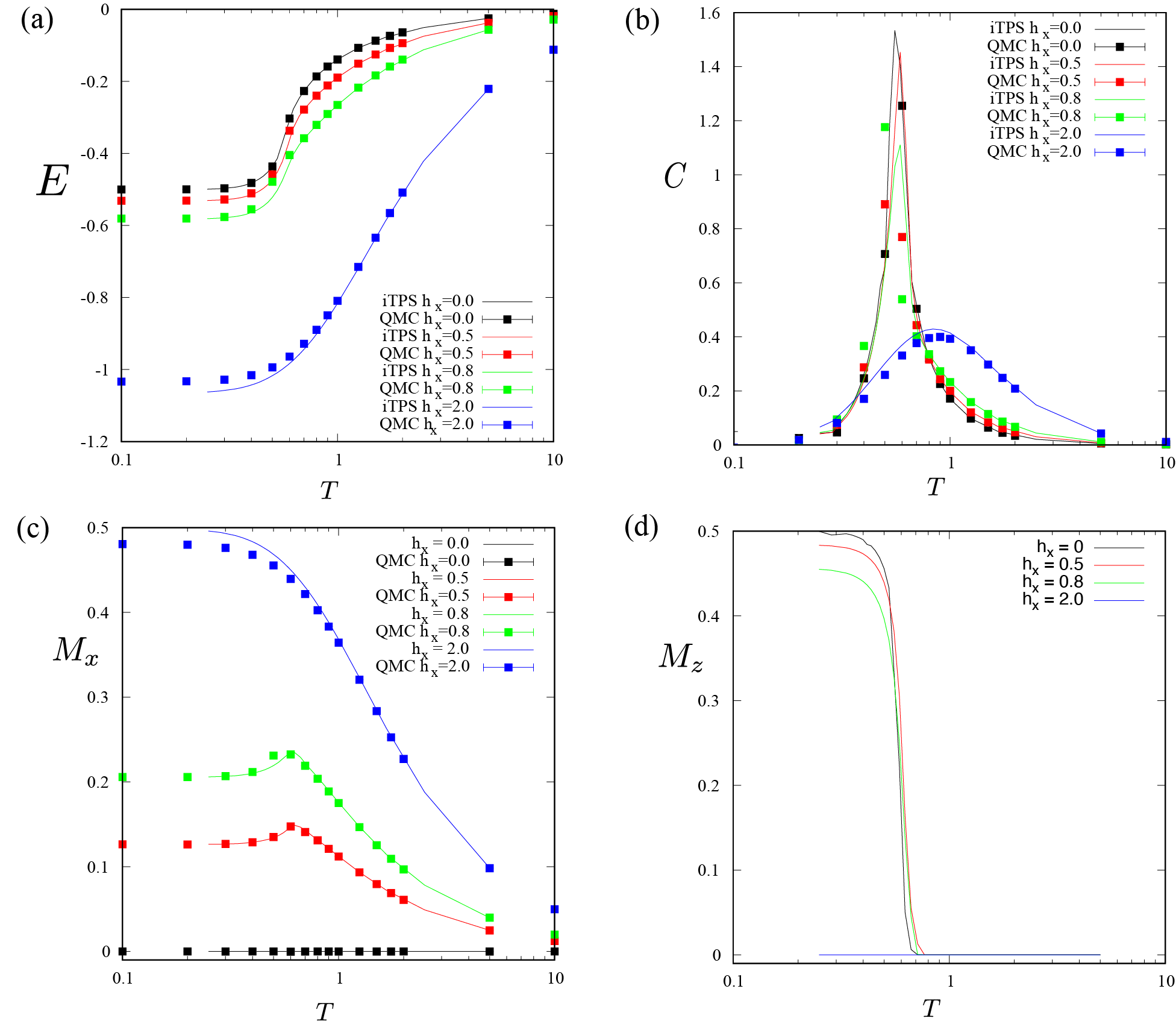
Fig. 4.4 Graphs for the finite temperature calculations of the Ising model: (a) energy, (b) heat capacity, (c) transverse magnetization, and (d) longitudinal magnetization. The vertical axis represents the physical quantity, and the horizontal axis denotes temperature. Curves are results by TeNeS and squares are results by DSQSS/dla (longitudinal magnetization is zero from symmetry).