4.1. Ising model with transverse magnetic field

This section presents an example of calculation when the transverse magnetic field is applied to the Ising model. By changing the variable G in the input file, the magnitude of the transverse magnetic field will be modified. For example, when the transverse magnetic field is 0, the input file becomes

[parameter]
[parameter.tensor]
D  = 2     # tensor_dim
CHI  = 10  # env_dim

[parameter.simple_update]
num_step = 1000
tau = 0.01

[parameter.ctm]
iteration_max = 10

[lattice]
type = "square lattice"
L_sub = [2,2]

[model]
type = "spin"
Jz = -1.0
Jx = 0.0
Jy = 0.0
G = 0.0

In this case, since Jz = -1.0 , the ferro magnetic state becomes the ground state at G=0. When the input file name is simple.toml , type the following commands to execute tenes :

$ tenes_simple simple.toml
$ tenes input.toml

Then, the following logs are output to the standard output.

Start simple update
Start calculating observables
Start updating environment
Start calculating local operators
Save site observables to output/site_obs.dat
Start calculating energy
Save energy to output/energy.dat
Start calculating NN correlation
Save NN correlation to output/neighbor_obs.dat
Save elapsed times to output/time.dat

Energy = -0.5
Local operator 0 = 0.5
Local operator 1 = 1.90794709356e-11

time simple update = 3.21127
time full update   = 0
time environmnent  = 0.875561
time observable    = 0.132412

The execution status of each process is displayed first. After finishing the calculation, Energy and the local operators Local operator 0 (<Sz>), Local operator 1 (<Sx>) are outputted, respectively. Finally, time is printed to show the calculation time (Time unit is seconds). In the output folder, energy.dat, parameters.dat, time.dat, neighbor_obs.dat, site_obs.dat are outputted. For details about each output file, see the file formats. The value of <Sz> can be extracted from the value following the 0 0 component of site_obs.dat or the Local operator 0 in the standard output. By changing G in increments of 0.1 from 0 to 2.0 and running tenes_simple and tenes, the following result is obtained.

As an exapmle of the sample script, tutorial_example.py , tutorial_read.py are prepared in the sample/01_transverse_field_ising directory. The calculation will be done by typing the following command:

$ python tutorial_example.py

For MacBook2017 (1.4 GHz Intel Core i7), the calculation was finished in a few minutes. By typing the following command, G, energy, <Sz> and <Sx> are ouputted in the standard output:

$ python tutorial_read.py

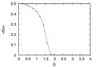
As you can see from the figure, with increasing G, the <Sz> decreases gradually from 0.5 to 0.