4.1. Calculation of the degree of inversion of Mg, Al atoms in an ionic crystal MgAl2O4
Input files are available from examples/standard/spinel .
4.1.1. Example by using QuantumESPRESSO
Preparing the input files for abICS
The input file of abICS is input_qe.toml .
[replica]
nreplicas = 2
nprocs_per_replica = 1

kTstart = 1000.0
kTend = 1200.0

nsteps = 5  # Number of steps for sampling
RXtrial_frequency = 1
sample_frequency = 1
print_frequency = 1
[replica] is a section for specifying parameters of the exchange Monte Carlo method.
In this example, the number of the replicas is 2 and the number of the steps is 5.
[solver]
type = 'qe'
path= './pw.x'
base_input_dir = './baseinput'
perturb = 0.0
run_scheme = 'mpi_spawn'
[solver] is a section for specifying a solver program.
This examples set type as qe in order to use Quantum ESPRESSO (QE).
path specifies the path to pw.x, the SCF energy solver of QE.
The directory that contains the input parameter files specific to each solver is given as ./baseinput using base_input_dir.
perturb is a random parameter that shifts atomic positions for structural optimization, but in this example it is set to 0 not to perform structural optimization.
abICS starts pw.x with MPI_Comm_spawn, so give mpi_spawn as run_scheme.
[config]
unitcell = [[8.1135997772, 0.0000000000, 0.0000000000],
            [0.0000000000, 8.1135997772, 0.0000000000],
            [0.0000000000, 0.0000000000, 8.1135997772]]
supercell = [1,1,1]
[config] is the atomic position section.
Specify the simulation cell (In units of angstrom) to be simulated by unitcell and supercell.
[[config.base_structure]]
type = "O"
coords = [
     [0.237399980, 0.237399980, 0.237399980],
     [0.762599945, 0.762599945, 0.762599945],
     [0.512599945, 0.012600004, 0.737399936],
     [0.487399966, 0.987399936, 0.262599975],
     [0.012600004, 0.737399936, 0.512599945],
     [0.987399936, 0.262599975, 0.487399966],
     [0.737399936, 0.512599945, 0.012600004],
     [0.262599975, 0.487399966, 0.987399936],
     [0.987399936, 0.487399966, 0.262599975],
     [0.012600004, 0.512599945, 0.737399936],
     [0.487399966, 0.262599975, 0.987399936],
     [0.512599945, 0.737399936, 0.012600004],
     [0.262599975, 0.987399936, 0.487399966],
     [0.737399936, 0.012600004, 0.512599945],
     [0.237399980, 0.737399936, 0.737399936],
     [0.762599945, 0.262599975, 0.262599975],
     [0.512599945, 0.512599945, 0.237399980],
     [0.487399966, 0.487399966, 0.762599945],
     [0.012600004, 0.237399980, 0.012600004],
     [0.987399936, 0.762599945, 0.987399936],
     [0.987399936, 0.987399936, 0.762599945],
     [0.012600004, 0.012600004, 0.237399980],
     [0.487399966, 0.762599945, 0.487399966],
     [0.512599945, 0.237399980, 0.512599945],
     [0.737399936, 0.237399980, 0.737399936],
     [0.262599975, 0.762599945, 0.262599975],
     [0.237399980, 0.512599945, 0.512599945],
     [0.762599945, 0.487399966, 0.487399966],
     [0.762599945, 0.987399936, 0.987399936],
     [0.237399980, 0.012600004, 0.012600004],
     [0.737399936, 0.737399936, 0.237399980],
     [0.262599975, 0.262599975, 0.762599945],
     ]
[[config.base_structure]] is a section that specifies the atoms that should not be moved in the Monte Carlo calculation.
type is the name of the atom and coords is the fraction coordinate where the atom is located.
coords can be used to give not only a list of lists but also a string representing a numeric matrix with three columns separated by white space and as many rows as there are atoms.
[[config.defect_structure]]
coords = [
     [0.000000000, 0.000000000, 0.000000000],
     [0.749999940, 0.249999985, 0.499999970],
     [0.249999985, 0.749999940, 0.499999970],
     [0.249999985, 0.499999970, 0.749999940],
     [0.749999940, 0.499999970, 0.249999985],
     [0.499999970, 0.749999940, 0.249999985],
     [0.499999970, 0.249999985, 0.749999940],
     [0.000000000, 0.499999970, 0.499999970],
     [0.749999940, 0.749999940, 0.000000000],
     [0.249999985, 0.249999985, 0.000000000],
     [0.249999985, 0.000000000, 0.249999985],
     [0.749999940, 0.000000000, 0.749999940],
     [0.499999970, 0.000000000, 0.499999970],
     [0.000000000, 0.749999940, 0.749999940],
     [0.000000000, 0.249999985, 0.249999985],
     [0.499999970, 0.499999970, 0.000000000],
     [0.374999970, 0.374999970, 0.374999970],
     [0.624999940, 0.624999940, 0.624999940],
     [0.374999970, 0.874999940, 0.874999940],
     [0.624999940, 0.124999993, 0.124999993],
     [0.874999940, 0.874999940, 0.374999970],
     [0.124999993, 0.124999993, 0.624999940],
     [0.874999940, 0.374999970, 0.874999940],
     [0.124999993, 0.624999940, 0.124999993],
     ]
[[config.defect_structure]] is the section for specifying the positions of the atoms you want to move in the Monte Carlo calculation.
[[config.defect_structure.groups]]
name = 'Al'
# species = ['Al']    # default
# coords = [[[0,0,0]]]  # default
num = 16
[[config.defect_structure.groups]]
name = 'Mg'
# species = ['Mg']    # default
# coords = [[[0,0,0]]]  # default
num = 8
[[config.defect_structure.groups]] is the section for specifying the name and number of atoms to be moved in the Monte Carlo calculation.
Scatter the 16 Al and 8 Mg atoms into the coordinates specified by [[config.defect_structure]].
Preparing the input file of QE
abICS generates the input files of the solver from the internal atomic structure, but information other than the structure, such as pseudopotential information, must be supplied by the user.
In the case of QE, such information is specified by scf.in in the directory specified by base_input_dir in the format of the input file of pw.x.
Based on this file, an input file with unit cells and atomic structure is automatically generated.
Notes - The pseudopotential directory
pseudo_dirmust be passed as an absolute path.~expands to the user’s home directory. -disk_iomust not benone.
Execution and analysis
See “How to use” section for information on setting the number of processes and options for running MPI.
mpiexec -np 2 abics input_qe.toml
After the abICS calculation, the degree of inversion (DOI: ratio of Al atoms where Mg atoms were originally located) is calculated.
To do this, use the scripts separateT.py and calc_DOI.py in the examples/standard/spinel directory.
First, use separateT.py to summarize the structure information for each replica by temperature:
mpiexec -np 2 python3 ./separateT.py input_qe.toml
The results are stored in the Tseparate directory.
If this directory already exists, the old one is moved to another directory Tseparate.DATE (DATE is the current datetime).
Next, calculate DOI by using calc_DOI.py:
mpiexec -np 2 python3 ./calc_DOI.py input_qe.toml
The results are stored in Tseparate/DOI_T.dat .
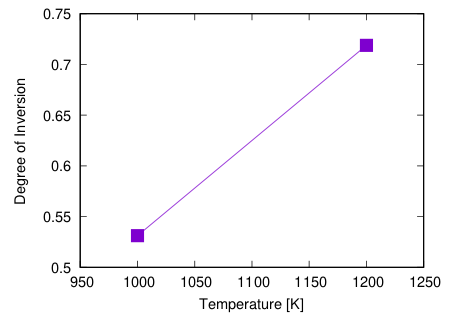
If you increase the number of replicas, you can calculate at various temperatures.
You can also get better results by increasing the number of steps.
The first number of samples to discard in Monte Carlo averaging can be specified by the value of throwout in the calc_DOI.py script.
For example, if you do with 17 replicas and 20 steps, the following result will be obtained
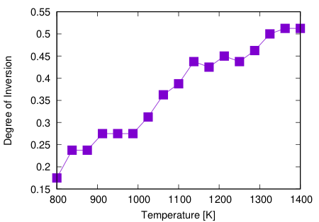
You can see that DOI increases as the temperature increases.