3. Usage
DSQSS provides an input file creation tool dsqss_pre.py .
This section briefly explains how to run DSQSS using this tool.
In DSQSS/DLA, it is also possible for users to define complex models and execute them.
For details, see User’s manual of DSQSS/DLA .
3.1. Make an input file
To run dsqss_pre.py, a text-based input file is needed.
An example of the input file is shown below.
[System]
solver = DLA
[Hamiltonian]
model_type = spin
M = 1
J = 1.0
F = 0.0
[Lattice]
lattice_type = square
D = 1
L = 8
Beta = 10
[Parameter]
NPRE = 1000
NTHERM = 1000
NMCS = 1000
NSET = 10
SEED = 31415
NVERMAX = 10000000
algfile = algorithm.xml
latfile = lattice.xml
outfile = sample.log
In the input file, specify the parameters that are divided into four categories.
Each parameter is specified in the form keyword = parameter.
System section
Set solvers with
solveras the keyword. Solvers can be selected fromDLAorPMWA.Hamiltonian section
Specify the system type (spin or boson) and the parameters to construct the Hamiltonian.
Parameter Solver Type Default Remarks model_typeCommon str spin spinorboson.
model_type = spin
Parameter Solver Type Default Remarks MDLA int 1 The number of sub-spins on each site. FDLA double 0.0 The magnetic field in the pair Hamiltonian. ( = \(H/z\) if the field \(H\) is shared equally by all pairs, where \(z = 4\) for a two-dimensional square lattice. ). JDLA double 1.0 The coupling constant \(J\) (positive for ferromagnets, negative for anti-magnets). JxyPMWA double 0.0 The coupling constant \(J_{xy}\) (positive for ferromagnets, negative for anti-magnets). JzPMWA double 0.0 The coupling constant \(J_{z}\) (positive for ferromagnets, negative for anti-magnets). hPMWA double 0.0 The longitudinal magnetic field (not depend on \(z\)). GammaPMWA double 0.0 The transverse magnetic field (not depend on \(z\)).
model_type = boson
Parameter Solver Type Default Remarks tCommon double 1.0 The hopping constant. UCommon double 0.0 The on-site interaction (positive for repulsive). VCommon double 0.0 The nearest neighbor interaction (positive for repulsive). MDLA int 1 The maximum number of bosons on each site. FDLA double 0.0 The chemical potential in the pair Hamiltonian ( = \(H/z\) if the field \(H\) is the field per site and \(H\) is shared equally by all pairs, e.g., \(F = H/4\) for a square lattice. ) muPMWA double 0.0 The chemical potential. GammaPMWA double 0.0 The source term ( the coefficient of \(b_i^{\dagger}+b_i\) ).
For details of the parameters constituting the Hamiltonian,
see the section for input files of hamgen_B or hamgen_H for DSQSS/DLA.
For DSQSS/PMWA , see the section for input file.
- Lattice section
This section specifies the lattice type and inverse temperature.
Parameter Type Default Remarks lattice_typestr square Select squareortriangularforDLA. ForPMWA, onlysquarecan be selected.Dint The number of dimension. Lint The liner size of the lattice. Specify the size of the Ddimensional space, separated by , for example, in the case of a lattice of 2D \(2 \times 4\), specify it asL = 2, 4.Betadouble 10.0 Inverse temperature NLdivint 1 ( for DSQSS/PMWA): The devision number for the lattice.NBdivint 1 ( for DSQSS/PMWA): The devision number forBeta.
- Parameter section
In this section, the calculation condition is specified. Set the parameters using keywords common to the input files ofDSQSS / DLAandDSQSS / PMWA. Please refer to the input file of each solver for details of defined parameters.
3.2. Execution
After making the input file, input files for the solver are generated by typing the following command (input file name is set as “std.in” in the following).
$ dsqss_pre.py -i std.in
For DSQSS/DLA , algorithm.xml, hamiltonian.xml, lattice.xml, param.in are generated.
For DSQSS/PMWA, lattice.xml, param.in are generated.
To execute the solver, see the end line of standard output of dsqss_pre.py
:
Please type: xxxxxx
where xxxxxx is the command for the execution (for example, DLA_H param.in).
To use MPI, add mpirun -np 8 in the front of xxxxxx (8 is the number of the processes to be used for parallelization).
DSQSS/DLA specifies the number of parallel random numbers,
DSQSS/PMWA specifies the product of the number of parallel random numbers
and the total number of divisions (product of space division number and imaginary time division number) as the number of processes.
Details of the output files after calculations are described in the tutorial / output result of each solver, so please refer to that.
3.3. Flow of Monte Carlo calculation
In Fig. 3.1 , the flow of Monte Carlo calculation is shown.
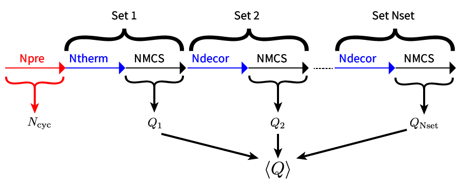
Fig. 3.1 Schematic figure for the flow of Monte Carlo calculation and the parameters for Monte Carlo steps
DSQSS defines 1 MC step from generation of worm head pair to disappearance and
defines 1 MC sweep as \(N_\text{cyc}\) MC step (even if generation of worm head pair fails, it is counted as 1 MC step.)
The value of \(N_\text{cyc}\) is determined by the initial NPRE MC step.
After determining \(N_\text{cyc}\) ,
Simulation of the NTHERM MC sweep is performed as an initial relaxation phase,
and the simulation of NMCS MC sweep continues as a physical quantity measurement phase.
A NDECOR MC sweep simulation is performed as an autocorrelation reduction phase
between one physical quantity measurement phase and the next physical quantity measurement process phase.
One set consists of two phases, the initial relaxation phase and the physical quantity measurement phase,
or the autocorrelation reduction phase and the physical quantity measurement phase,
and the whole simulation includes NSET sets.
Expected value of physical quantity \(\langle Q \rangle\) and error \(\sigma_Q\)
can be obtained as the mean and standard error of the physical quantity obtained from each of the NSET sets.