Optimization by Nelder-Mead method
In this section, we will explain how to calculate the inverse problem of analyzing atomic coordinates from diffraction data using the Nelder-Mead method. The specific calculation procedure is as follows.
Preparation of the reference file
Prepare the reference file to be matched (in this tutorial, it corresponds to
experiment.txtdescribed below).Perform calculations on the bulk part of the surface structure.
Copy
bulk.exetosample/sim-trhepd-rheed/minsearchand run the calculation.Run the main program
Run the calculation using
src/py2dmat_main.pyto estimate the atomic coordinates.
In the main program, the Nelder-Mead method (using scipy.optimize.fmin) is used. ) to find the parameter that minimizes the deviation (R-value) between the intensity obtained using the solver (in this case surf.exe) and the intensity listed in the reference file (experiment.txt).
Location of the sample files
The sample files are located in sample/py2dmat/sim-trhepd-rheed/single_beam/minsearch.
The following files are stored in the folder.
bulk.txtInput file of
bulk.exe.experiment.txt,template.txtReference file to proceed with calculations in the main program.
ref.txtA file containing the answers you want to seek in this tutorial.
input.tomlInput file of the main program.
prepare.sh,do.shScript prepared for doing all calculation of this tutorial
The following sections describe these files and then show the actual calculation results.
The reference file
The template.txt file is almost the same format as the input file for surf.exe.
The parameters to be run (such as the atomic coordinates you want to find) are rewritten as value_* or some other appropriate string.
The following is the content of template.txt.
2                                    ,NELMS,  -------- Ge(001)-c4x2
32,1.0,0.1                           ,Ge Z,da1,sap
0.6,0.6,0.6                          ,BH(I),BK(I),BZ(I)
32,1.0,0.1                           ,Ge Z,da1,sap
0.4,0.4,0.4                          ,BH(I),BK(I),BZ(I)
9,4,0,0,2, 2.0,-0.5,0.5               ,NSGS,msa,msb,nsa,nsb,dthick,DXS,DYS
8                                    ,NATM
1, 1.0, 1.34502591  1       value_01   ,IELM(I),ocr(I),X(I),Y(I),Z(I)
1, 1.0, 0.752457792 1       value_02
2, 1.0, 1.480003343 1.465005851     value_03
2, 1.0, 2   1.497500418     2.281675
2, 1.0, 1   1.5     1.991675
2, 1.0, 0   1       0.847225
2, 1.0, 2   1       0.807225
2, 1.0, 1.009998328 1       0.597225
1,1                                  ,(WDOM,I=1,NDOM)
In this input file, value_01, value_02, and value_03 are used.
In the sample folder, there is a reference file ref.txt to know if the atomic positions are estimated correctly. The contents of this file are
fx = 7.382680568652868e-06
z1 = 5.230524973874179
z2 = 4.370622919269477
z3 = 3.5961444501081647
value_0x corresponds to z_x (x=1, 2, 3).
fx is the optimal value of the objective function.
The experiment.txt is a file that is used as a reference in the main program, and is equivalent to convolution.txt, which is calculated by putting the parameters in ref.txt into template.txt and following the same procedure as in the tutorial on direct problems. (Note that the input files for bulk.exe and suft.exe are different from those in the sequential problem tutorial.)
Input file
In this section, we will prepare the input file input.toml for the main program.
The details of input.toml can be found in the input file.
This section describes the contents of input.toml in the sample file.
[base]
dimension = 3

[solver]
name = "sim-trhepd-rheed"

[solver.config]
calculated_first_line = 5
calculated_last_line = 74
row_number = 2

[solver.param]
string_list = ["value_01", "value_02", "value_03" ]
degree_max = 7.0

[solver.reference]
path = "experiment.txt"
first = 1
last = 70

[algorithm]
name = "minsearch"
label_list = ["z1", "z2", "z3"]

[algorithm.param]
min_list = [0.0, 0.0, 0.0]
max_list = [10.0, 10.0, 10.0]
initial_list = [5.25, 4.25, 3.50]
First, [base] section is explained.
The
dimensionis the number of variables to be optimized, in this case3since we are optimizing three variables as described intemplate.txt.
The [solver] section specifies the solver to be used inside the main program and its settings.
The
nameis the name of the solver you want to use, which in this tutorial issim-trhepd-rheed, since we will be using it for our analysis.
The solver can be configured in the subsections [solver.config], [solver.param], and [solver.reference].
The [solver.config] section specifies options for reading the output file produced by the main program’s internal call, surf.exe.
The
calculated_first_linespecifies the first line to read from the output file.The
calculated_last_linespecifies the last line of the output file to be read.The
row_numberspecifies the number of columns in the output file to read.
The [solver.param] section specifies options for reading the output file produced by the main program’s internal call, surf.exe.
The
string_listis a list of variable names to be read intemplate.txt.degree_maxspecifies the maximum angle in degrees.
The [solver.reference] section specifies the location of the experimental data and the range to read.
The
pathspecifies the path where the experimental data is located.The
firstspecifies the first line of the experimental data file to read.The
endspecifies the last line of the experimental data file to read.
The [algorithm] section specifies the algorithm to use and its settings.
The
nameis the name of the algorithm you want to use, in this tutorial we will useminsearchsince we will be using the Nelder-Mead method.The
label_listis a list of label names to be added to the output ofvalue_0x(x=1,2,3).
The [algorithm.param] section specifies the range of parameters to search and their initial values.
The
min_listandmax_listspecify the minimum and maximum values of the search range, respectively.The
initial_listspecifies the initial values.
Other parameters, such as convergence judgments used in the Nelder-Mead method, can be done in the [algorithm] section, although they are omitted here because the default values are used.
See the input file chapter for details.
Calculation execution
First, move to the folder where the sample files are located (we will assume that you are directly under the directory where you downloaded this software).
cd sample/sim-trhepd-rheed/single_beam/minsearch
Copy bulk.exe and surf.exe.
cp ../../../../../sim-trhepd-rheed/src/TRHEPD/bulk.exe .
cp ../../../../../sim-trhepd-rheed/src/TRHEPD/surf.exe .
First, run bulk.exe to create bulkP.b.
./bulk.exe
After that, run the main program (the computation time takes only a few seconds on a normal PC).
python3 ../../../../src/py2dmat_main.py input.toml | tee log.txt
Then, the standard output will be seen as follows.
Read experiment.txt
z1 =  5.25000
z2 =  4.25000
z3 =  3.50000
[' 5.25000', ' 4.25000', ' 3.50000']
PASS : degree in lastline = 7.0
PASS : len(calculated_list) 70 == len(convolution_I_calculated_list)70
R-factor = 0.015199251773721183
z1 =  5.50000
z2 =  4.25000
z3 =  3.50000
[' 5.50000', ' 4.25000', ' 3.50000']
PASS : degree in lastline = 7.0
PASS : len(calculated_list) 70 == len(convolution_I_calculated_list)70
R-factor = 0.04380131351780189
z1 =  5.25000
z2 =  4.50000
z3 =  3.50000
[' 5.25000', ' 4.50000', ' 3.50000']
...
The z1, z2, and z3 are the candidate parameters at each step and the R-factor at that time.
The results of each step are also output to the folder Logxxxxx (where xxxxxx is the number of steps).
The final estimated parameters will be output to res.dat.
In the current case, the following result is obtained:
z1 = 5.230524973874179
z2 = 4.370622919269477
z3 = 3.5961444501081647
You can see that we get the same value as the correct answer data ref.txt.
Note that do.sh is available as a script for batch calculation.
In do.sh, it also compares the difference between res.txt and ref.txt.
Here is what it does, without further explanation.
sh ./prepare.sh

./bulk.exe

time python3 ../../../../src/py2dmat_main.py input.toml | tee log.txt

echo diff res.txt ref.txt
res=0
diff res.txt ref.txt || res=$?
if [ $res -eq 0 ]; then
  echo Test PASS
  true
else
  echo Test FAILED: res.txt and ref.txt differ
  false
fi
Visualization of calculation results
The data of the rocking curve at each step is stored in Logxxxx_00000001 (where xxxx is the index of steps) as RockingCurve.txt.
A tool draw_RC_double.py is provided to visualize this data.
In this section, we will use this tool to visualize the results.
cp 0/Log00000001_00000001/RockingCurve.txt RockingCurve_ini.txt
cp 0/Log00000062_00000001/RockingCurve.txt RockingCurve_con.txt
cp ../../../../script/draw_RC_double.py .
python draw_RC_double.py
Running the above will output RC_double.png.
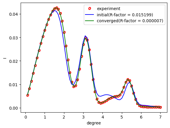
Fig. 2 Analysis using the Nelder-Mead method. The red circle represents the experimental value, the blue line represents the first step, and the green line represents the rocking curve obtained at the last step.
From the figure, we can see that the last step agrees with the experimental one.