Grid search

In this section, we will explain how to perform a grid-type search and analyze atomic coordinates from diffraction data. The grid type search is compatible with MPI. The specific calculation procedure is the same as for minsearch. However, it is necessary to prepare the data MeshData.txt to give the search grid in advance.

Location of the sample files

The sample files are located in sample/sim-trhepd-rheed/single_beam/mapper. The following files are stored in the folder

• bulk.txt

  Input file of bulk.exe

• experiment.txt , template.txt

  Reference file to proceed with calculations in the main program.

• ref_ColorMap.txt

  A file to check if the calculation was performed correctly (the answer to ColorMap.txt obtained by doing this tutorial).

• input.toml

  Input file of the main program.

• prepare.sh , do.sh

  Script prepared for bulk calculation of this tutorial.

Below, we will describe these files and then show the actual calculation results.

Reference file

The template.txt and experiment.txt are the same as in the previous tutorial (Nealder-Mead optimization). However, to reduce the computation time, the value is fixed to 3.5 instead of value_03, and the grid is searched in 2D. The actual grid to be searched is given in MeshData.txt. In the sample, the contents of MeshData.txt are as follows.

1 6.000000 6.000000
2 6.000000 5.750000
3 6.000000 5.500000
4 6.000000 5.250000
5 6.000000 5.000000
6 6.000000 4.750000
7 6.000000 4.500000
8 6.000000 4.250000
9 6.000000 4.000000
...

The first column is the serial number, and the second and subsequent columns are the values of value_0 , value_1 that go into template.txt, in that order.

Input file

This section describes the input file for the main program, input.toml. The details of input.toml can be found in the input file. The following is the content of input.toml in the sample file.

[base]
dimension = 2

[solver]
name = "sim-trhepd-rheed"

[solver.config]
calculated_first_line = 5
calculated_last_line = 74
row_number = 2

[solver.param]
string_list = ["value_01", "value_02" ]
degree_max = 7.0

[solver.reference]
path = "experiment.txt"
first = 1
last = 70

[algorithm]
name = "mapper"
label_list = ["z1", "z2"]

First, [base] section is explained.

• The dimension is the number of variables to be optimized, in this case 2 since we are optimizing two variables as described in template.txt.

The [solver] section specifies the solver to be used inside the main program and its settings.

• The name is the name of the solver you want to use, which in this tutorial is sim-trhepd-rheed, since we will be using it for our analysis.

The solver can be configured in the subsections [solver.config], [solver.param], and [solver.reference].

The [solver.config] section specifies options for reading the output file produced by the main program’s internal call, surf.exe.

• The calculated_first_line specifies the first line to read from the output file.

• The calculated_last_line specifies the last line of the output file to be read.

• The row_number specifies the number of columns in the output file to read.

The [solver.param] section specifies options for reading the output file produced by the main program’s internal call, surf.exe.

• The string_list is a list of variable names to be read in template.txt.

• degree_max specifies the maximum angle in degrees.

The [solver.reference] section specifies the location of the experimental data and the range to read.

• The path specifies the path where the experimental data is located.

• The first specifies the first line of the experimental data file to read.

• The end specifies the last line of the experimental data file to read.

The [algorithm] section specifies the algorithm to use and its settings.

• The name is the name of the algorithm you want to use, in this tutorial we will use mapper since we will be using grid-search method.

• The label_list is a list of label names to be attached to the output value_0x (x=1,2).

For details on other parameters that can be specified in the input file, please see the Input File chapter.

Calculation execution

First, move to the folder where the sample files are located (we will assume that you are directly under the directory where you downloaded this software).

cd sample/sim-trhepd-rheed/single_beam/minsearch

Copy bulk.exe and surf.exe.

cp ../../../../../sim-trhepd-rheed/src/TRHEPD/bulk.exe .
cp ../../../../../sim-trhepd-rheed/src/TRHEPD/surf.exe .

First, run bulk.exe to create bulkP.b.

./bulk.exe

After that, run the main program (the computation time takes only a few seconds on a normal PC).

mpiexec -np 2 python3 ../../../../src/py2dmat_main.py input.toml | tee log.txt

Here, the calculation using MPI parallel with 2 processes will be done. When executed, a folder for each rank will be created, and a subfolder Log%%%%% (where %%%%% is the grid id) will be created under it. (The grid id is assigned to the number in MeshData.txt). The standard output will be seen like this.

Iteration : 1/33
Read experiment.txt
mesh before: [1.0, 6.0, 6.0]
z1 =  6.00000
z2 =  6.00000
[' 6.00000', ' 6.00000']
PASS : degree in lastline = 7.0
PASS : len(calculated_list) 70 == len(convolution_I_calculated_list)70
R-factor = 0.04785241875354398
...

The z1 and z2 are the candidate parameters for each mesh and the R-factor at that time. Finally, the R-factor calculated for all the points on the grid will be output to ColorMap.txt. In this case, the following results will be obtained.

6.000000 6.000000 0.047852
6.000000 5.750000 0.055011
6.000000 5.500000 0.053190
6.000000 5.250000 0.038905
6.000000 5.000000 0.047674
6.000000 4.750000 0.065919
6.000000 4.500000 0.053675
6.000000 4.250000 0.061261
6.000000 4.000000 0.069351
6.000000 3.750000 0.071868
6.000000 3.500000 0.072739
...

The first and second columns will contain the values of value_01 and value_02, and the third column will contain the R-factor. Note that do.sh is available as a script for batch calculation. In do.sh, it also compares the difference between res.txt and ref.txt. Here is what it does, without further explanation.

sh prepare.sh

./bulk.exe

time mpiexec -np 2 python3 ../../../../src/py2dmat_main.py input.toml

echo diff ColorMap.txt ref_ColorMap.txt
res=0
diff ColorMap.txt ref_ColorMap.txt || res=$?
if [ $res -eq 0 ]; then
  echo TEST PASS
  true
else
  echo TEST FAILED: ColorMap.txt and ref_ColorMap.txt differ
  false
fi

Visualization of calculation results

By seeing ColorMap.txt, we can estimate the region where the small parameters of R-factor are located. In this case, the following command will create a two-dimensional parameter space diagram ColorMapFig.png.

python3 plot_colormap_2d.py

Looking at the generated figure, we can see that it has a minimum value around (5.25, 4.25).

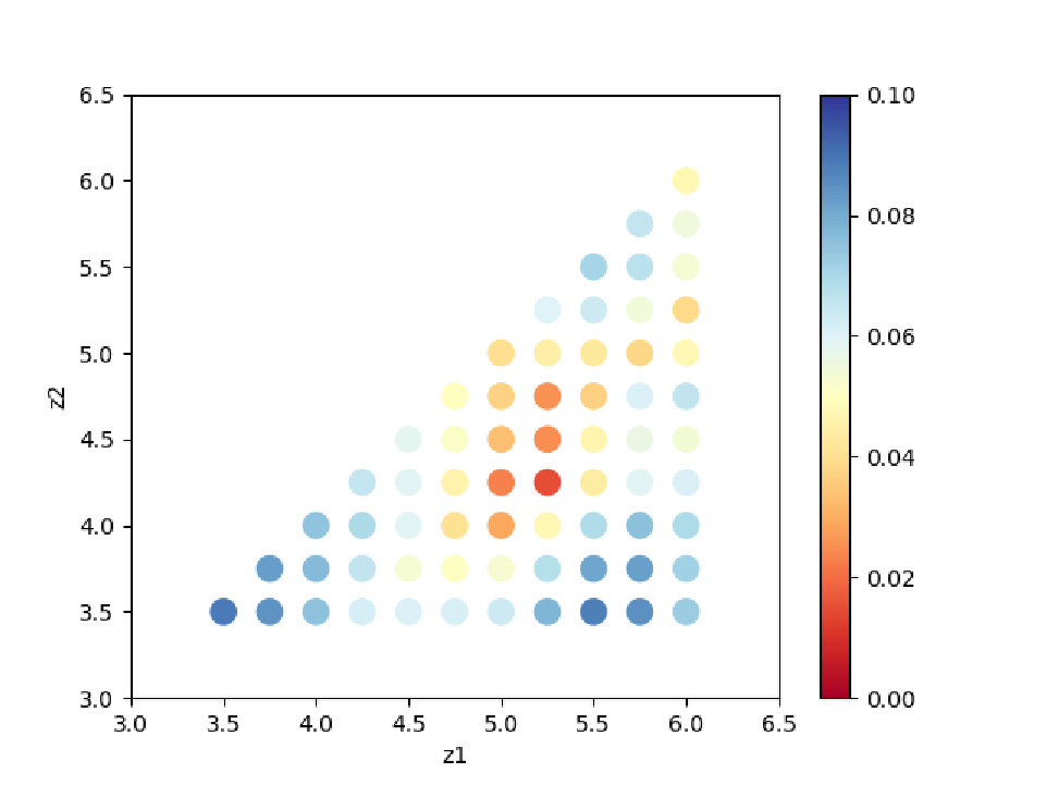
Fig. 3 R-factor on a two-dimensional parameter space.

RockingCurve.txt is stored in each subfolder. By using it, you can compare the results with the experimental values following the procedure in the previous tutorial.