CT-QMC: TRIQS/cthyb

Install

Follow the installation guide in TRIQS/cthyb.

Note

• Be sure to use the same C++ compiler as the one used to build the TRIQS library.

• If you want to treat the spin-orbit coupling in TRIQS/cthyb solver, it must be built with the following CMake options:

  -DLocal_hamiltonian_is_complex=ON -DHybridisation_is_complex=ON
  

Basic parameters for QMC

The accuracy of the TRIQS/cthyb calculation depends on mainly the following three parameters.

• n_cycles{int}

  The number of QMC cycles for computing any quantities. The numerical noise can be reduced by increasing this parameter.

  When we use the MPI parallelism, the total number of QMC cycle ( number-of-processes * n_cycles) affects the accuracy. Therefore, n_cycles in inverse proportion to the number of MPI processes keeps the accuracy.

• n_warmup_cycles{int}

  The number of QMC cycles for the thermalization before the above main calculation. If it is insufficient, the state to be computed may be different from the equilibrium state.

  This parameter is independent of the MPI parallelism.

• length_cycle{int}

  Each QMC cycles have sub-cycles. The length of this sub-cycle should be long enough to escape from the auto-correlation.

  This parameter is independent of the MPI parallelism.

The computational time is proportional to length_cycle*(n_cycles+n_warmup_cycles). The following script is an example to describe the procedure for searching appropriate QMC parameter.

#!/bin/bash

cat > pre.ini <<EOF
[model]
seedname = bethe
lattice = bethe
norb = 1
nelec = 1.0
t = 1.0
kanamori = [(4.0, 0.0, 0.0)]

[system]
beta = 40.0
nk = 100

[impurity_solver]
name = TRIQS/cthyb
n_warmup_cycles{int} = 10000
n_cycles{int} = 10000
length_cycle{int} = 100

[control]
max_step = 1
EOF

dcore_pre pre.ini

n_cycles[0]=3000;   n_warmup_cycles[0]=5000; length_cycle[0]=50
n_cycles[1]=10000;  n_warmup_cycles[1]=5000; length_cycle[1]=50
n_cycles[2]=30000;  n_warmup_cycles[2]=5000; length_cycle[2]=50
n_cycles[3]=100000; n_warmup_cycles[3]=5000; length_cycle[3]=50
n_cycles[4]=300000; n_warmup_cycles[4]=5000; length_cycle[4]=50
n_cycles[5]=300000; n_warmup_cycles[5]=5000; length_cycle[5]=100

for i in `seq 0 5`
do
    sed -e "/n_cycles/c n_cycles{int} = ${n_cycles[i]}" \
        -e "/n_wamup_cycles/c n_warmup_cycles{int} = ${n_wamup_cycles[i]}" \
        -e "/length_cycle/c length_cycle{int} = ${length_cycle[i]}" \
    pre.ini > dmft.ini
    mpiexec -np 4 dcore dmft.ini
    dcore_check dmft.ini --output bethe.pdf
    mv bethe_sigma.dat cyc${n_cycles[i]}_warm${n_warmup_cycles[i]}_len${length_cycle[i]}.dat
done

Then, we use gnuplot as

plot [0:10][-0.6:0] \
"cyc3000_warm5000_len50.dat" u 1:3 w l lw 3, \
"cyc10000_warm5000_len50.dat" u 1:3 w l lw 3, \
"cyc30000_warm5000_len50.dat" u 1:3 w l lw 3, \
"cyc100000_warm5000_len50.dat" u 1:3 w l lw 3, \
"cyc300000_warm5000_len50.dat" u 1:3 w l lw 3, \
"cyc300000_warm5000_len100.dat" u 1:3 w l lw 3

and obtain

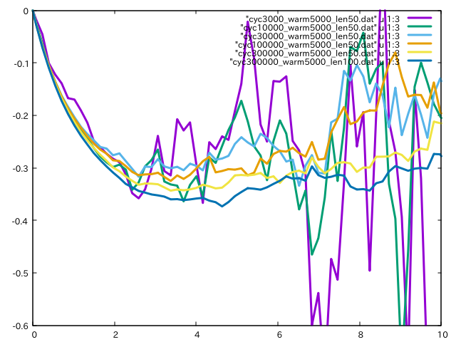
From this plot, we can see that both parameter settings are insufficient and we have to increase n_cycles or length_cycle or both of them (In almost cases, n_warmup_cycles has minor effect).

High-frequency tail fit

The self energy computed with QMC becomes noisy at the high frequency region. This high-frequency tail can be fitted by using the following function:

\[\Sigma_{\rm tail}(i \omega) \approx \frac{a_1}{\omega} + \frac{a_2}{\omega^2} + \frac{a_3}{\omega^3} + \cdots\]

We show the procedure for using this technique. The original input file (without tail-fit) is as follows (dmft.ini):

[model]
seedname = bethe
lattice = bethe
norb = 1
nelec = 1.0
t = 1.0
kanamori = [(4.0, 0.0, 0.0)]

[system]
beta = 40.0
nk = 100

[impurity_solver]
name = TRIQS/cthyb
n_warmup_cycles{int} = 10000
n_cycles{int} = 100000
length_cycle{int} = 50

[control]
max_step = 1

[tool]
omega_check = 30.0

We first execute the ordinary DMFT calculation:

$ dcore_pre dmft.ini
$ mpiexec -np 4 dcore dmft.ini
$ dcore_check dmft.ini --output bethe.pdf

Then, looking at the figure in bethe.pdf, we choose the energy range where the tail-fit is performed.

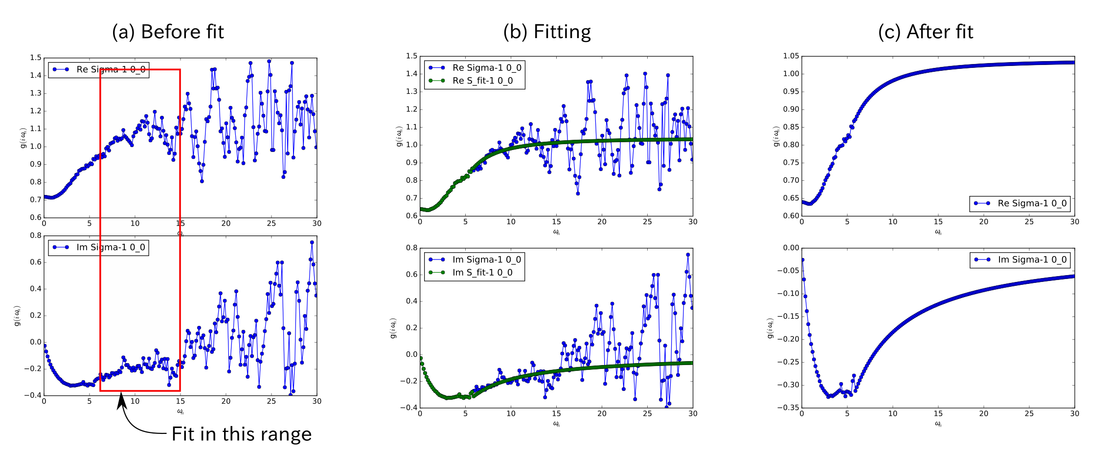
In this case, we choose energy range from 6 to 15 [red box in (a) in the above figure], and add the following parameters at the [system] block in the input file (not the solver parameter for the tail fit):

[system]
beta = 40.0
nk = 100
perform_tail_fit = True
fit_max_moment = 2
fit_min_w = 6.0
fit_max_w = 15.0

We run dcore_check again, and obtain the result as (b) in the above figure. If necessary, we repeat editing the input file and running dcore_check to refine the energy range. After the energy range is fixed, we again perform the QMC calculation by dcore. The final result looks like (c) in the above figure.

Multi-band system

For the multi-band systems, we have to include the two-pairs insertion/removal move in the QMC cycles as

[impurity_solver]
name = TRIQS/cthyb
move_double{bool} = True

because these moves are disabled in the default setting.

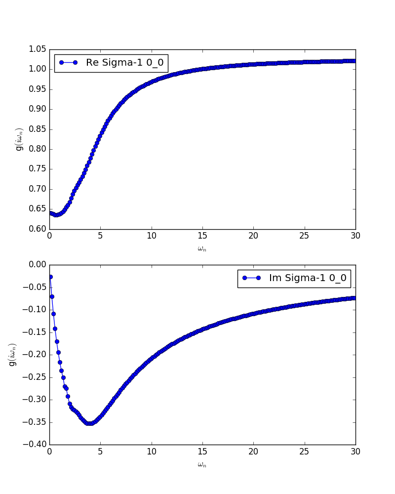
Pade approximation for DOS and spectrum function

To obtain spectral functions, we need to perform analytical continuation from Matsubara frequency to real frequency. Currently, the Pade approximation is the only choice for the analytical continuation.

There is one control parameter for Pade approximation, omega_pade in the [tool] block. It specifies an energy cutoff for Matsubara frequency. A reasonable choice of omega_pade is the maximum frequency before the self energy becomes noisy. For example, in the case of figure (a) above, we can find that omega_pade=4.0 is reasonable.

Legendre filter

Warning

Do not use it together with the tail-fit.

This is another technique to reduce the high-frequency noise. In this method, we expand the Green’s function at the imaginary time with a series of the Legendre polynomials, and ignore the higher order polynomials.

This scheme is activated when we specify the input parameter n_l (the number of polynomial included) in the [system] block as

[system]
beta = 40.0
nk = 100
n_l = 30

When we use the Legendre filter, we should check that how many polynomials have to be included. For this purpose, we first perform a calculation with a large number of Legendre polynomials (e.g. n_l=80) and check how the coefficient decays.

For examples, we run the bash script as

#!/bin/bash

cat > pre.ini <<EOF
[model]
seedname = bethe
lattice = bethe
norb = 1
nelec = 1.0
t = 1.0
kanamori = [(4.0, 0.0, 0.0)]

[system]
beta = 40.0
nk = 100
n_l = 30

[impurity_solver]
name = TRIQS/cthyb
n_warmup_cycles{int} = 10000
n_cycles{int} = 10000
length_cycle{int} = 100

[control]
max_step = 1
EOF

dcore_pre pre.ini

n_cycles[0]=3000;   n_warmup_cycles[0]=5000; length_cycle[0]=50
n_cycles[1]=10000;  n_warmup_cycles[1]=5000; length_cycle[1]=50
n_cycles[2]=30000;  n_warmup_cycles[2]=5000; length_cycle[2]=50
n_cycles[3]=100000; n_warmup_cycles[3]=5000; length_cycle[3]=50
n_cycles[4]=300000; n_warmup_cycles[4]=5000; length_cycle[4]=50
n_cycles[5]=300000; n_warmup_cycles[5]=5000; length_cycle[5]=100

for i in `seq 0 5`
do
    sed -e "/n_cycles/c n_cycles{int} = ${n_cycles[i]}" \
        -e "/n_wamup_cycles/c n_warmup_cycles{int} = ${n_wamup_cycles[i]}" \
        -e "/length_cycle/c length_cycle{int} = ${length_cycle[i]}" \
    pre.ini > dmft.ini
    mpiexec -np 4 dcore dmft.ini
    dcore_check dmft.ini --output bethe.pdf
    mv bethe_legendre.dat l_cyc${n_cycles[i]}_warm${n_warmup_cycles[i]}_len${length_cycle[i]}.dat
done

Then, we use GnuPlot as

set xlabel "Order of polynomial"
set ylabel "Coefficient"
set logscale y
plot \
"l_cyc3000_warm5000_len50.dat" u 1:(abs($2)) w l lw 3, \
"l_cyc10000_warm5000_len50.dat" u 1:(abs($2)) w l lw 3, \
"l_cyc30000_warm5000_len50.dat" u 1:(abs($2)) w l lw 3, \
"l_cyc100000_warm5000_len50.dat" u 1:(abs($2)) w l lw 3, \
"l_cyc300000_warm5000_len50.dat" u 1:(abs($2)) w l lw 3, \
"l_cyc300000_warm5000_len100.dat" u 1:(abs($2)) w l lw 3

and obtain

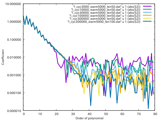
Finally, we choose the following setting:

[model]
seedname = bethe
lattice = bethe
norb = 1
nelec = 1.0
t = 1.0
kanamori = [(4.0, 0.0, 0.0)]

[system]
beta = 40.0
nk = 100
n_l = 30

[impurity_solver]
name = TRIQS/cthyb
n_warmup_cycles{int} = 5000
n_cycles{int} = 300000
length_cycle{int} = 100

[control]
max_step = 1

[tool]
omega_check = 30.0

and obtain