Wanniernization using OpenMX
OpenMX is a first-principles program package based on the numerical localized basis set and pseudopotentials. OpenMX itself can generate hopping parameter in the wannier90 format. In this tutorial, we demonstrate the calculation of SrVO3.
Note
This tutorial requires large computational resources or long simulation time.
SCF computation and Wannier with OpenMX
#
# File Name
#
System.CurrrentDirectory         ./    # default=./
System.Name                      SrVO3
level.of.stdout                   1    # default=1 (1-3)
level.of.fileout                  1    # default=1 (0-2)
data.path                 /mnt/c/Users/kawamuura/program/openmx-eca/DFT_DATA13/
#
# Definition of Atomic Species
#
Species.Number       4
<Definition.of.Atomic.Species
  Sr  Sr10.0-s2p2d1  Sr_PBE13
   V  V6.0-s2p1d1     V_PBE13
   O  O7.0-s2p2d1     O_PBE13
proj  V6.0-s1p1d1     V_PBE13
Definition.of.Atomic.Species>
#
# Atoms
#
Atoms.Number         5
Atoms.SpeciesAndCoordinates.Unit   FRAC # Ang|AU
<Atoms.SpeciesAndCoordinates
1  Sr   0.0  0.0  0.0  5.0  5.0
2   V   0.5  0.5  0.5  6.5  6.5
3   O   0.5  0.0  0.5  3.0  3.0
4   O   0.0  0.5  0.5  3.0  3.0
5   O   0.5  0.5  0.0  3.0  3.0
Atoms.SpeciesAndCoordinates>
Atoms.UnitVectors.Unit  AU  # Ang|AU
<Atoms.UnitVectors
7.29738  0.00000  0.00000
0.00000  7.29738  0.00000
0.00000  0.00000  7.29738
Atoms.UnitVectors>
#
# SCF or Electronic System
#
scf.XcType                 GGA-PBE     # LDA|LSDA-CA|LSDA-PW|GGA-PBE
scf.SpinPolarization        Off         # On|Off|NC
scf.maxIter                  50        # default=40
scf.EigenvalueSolver       band        # DC|GDC|Cluster|Band
scf.Kgrid                  8 8 8       # means n1 x n2 x n3
scf.Mixing.Type           rmm-diisk    # Simple|Rmm-Diis|Gr-Pulay|Kerker|Rmm-Diisk
scf.Init.Mixing.Weight     0.20        # default=0.30
scf.Min.Mixing.Weight      0.001       # default=0.001
scf.Max.Mixing.Weight      0.500       # default=0.40
scf.Mixing.History          7          # default=5
scf.Mixing.StartPulay       7          # default=6
scf.Mixing.EveryPulay       1          # default=6
scf.criterion             1.0e-7       # default=1.0e-6 (Hartree)
orbitalOpt.Force.Skip       on
#scf.restart                on
#
# Band dispersion
#
Band.dispersion              on        # on|off, default=off
Band.Nkpath  4
<Band.kpath
15  0.0  0.0  0.0    0.5  0.0  0.0  g  X
15  0.5  0.0  0.0    0.5  0.5  0.0  X  M
15  0.5  0.5  0.0    0.0  0.0  0.0  M  g
15  0.0  0.0  0.0    0.5  0.5  0.5  g  R
Band.kpath>
#
# Wannier
#
Wannier.Func.Calc on #default off
Wannier.Func.Num 3 #no default
Wannier.Outer.Window.Bottom  -1.5
Wannier.Outer.Window.Top      7.0
Wannier.Inner.Window.Bottom  -1.5
Wannier.Inner.Window.Top      1.2
Wannier.Initial.Projectors.Unit FRAC
<Wannier.Initial.Projectors
proj-dxy 0.5 0.5 0.5  0.0 0.0 1.0  1.0 0.0 0.0
proj-dxz 0.5 0.5 0.5  0.0 0.0 1.0  1.0 0.0 0.0
proj-dyz 0.5 0.5 0.5  0.0 0.0 1.0  1.0 0.0 0.0
Wannier.Initial.Projectors>
Wannier.Interpolated.Bands             on
Wannier.Function.Plot                  on         # default off
Wannier.Function.Plot.SuperCells      1 1 1       # default=0 0 0
$ openmx scf.dat
Then, convert the OpenMX output to the wannier90 format.
It can be performed with openmx2dcore utility as:
$ openmx2dcore.py SrVO3 srvo3
DMFT calculation
[model]
lattice = wannier90
seedname = srvo3
nelec = 1.0
ncor = 1
norb = 3
kanamori = [(3.419, 2.315, 0.530)]
bvec=[(1.627091,0.0,0.0),(0.0,1.627091,0.0),(0.0,0.0,1.627091)]

[system]
nk0 = 16
nk1 = 16
nk2 = 16
beta = 40.0
mu = 0.0
with_dc = True
perform_tail_fit = True
fit_max_moment = 8
fit_min_w = 5.0
fit_max_w = 19.0

[impurity_solver]
name = TRIQS/cthyb
n_cycles{int} = 10000
n_warmup_cycles{int} = 10000
length_cycle{int} = 500
move_double{bool} = True

[control]
max_step = 8

[post.spectrum]
broadening = 0.1
nk_line = 50
knode=[(G,0.0,0.0,0.0),(X,0.5,0.0,0.0),(M,0.5,0.5,0.0),(G,0.0,0.0,0.0),(R,0.5,0.5,0.5)]

[post.anacont]
omega_max =2.0
omega_min =-2.0
Nomega = 400

[post.anacont.pade]
iomega_max = 5.0

[post.check]
omega_check = 30.0
Please see CT-QMC: TRIQS/cthyb for the details of the parameter setting.
Note
The parameter n_cycles{int} should be tuned in inverse proportion to the number of MPI processes.
The following result is obtained with 432 MPI processes at n_cycles{int} = 10000
(70 seconds per DMFT cycle on ISSP system B).
If we want to compute by using 32 MPI processes at the same accuracy,
n_cycles{int} should be 10000*432/32=135000.
DMFT setup: dcore_pre
$ dcore_pre srvo3.ini
Running self-consistent DMFT calculation: dcore
$ dcore srvo3.ini
Post-processing and data analysis: dcore_anacont and dcore_spectrum
$ dcore_anacont srvo3.ini
$ dcore_spectrum srvo3.ini
$ cd post
$ sed -e "s/every 10/every 1/g" akw.gp
$ gnuplot akw.gp
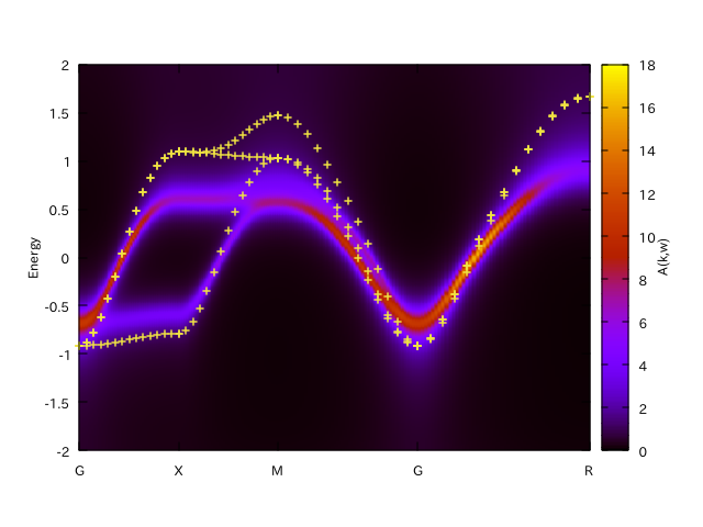
“+” indicates the original band structure.