5.1. Tutorial
To use H-wave for the calculation of Random Phase Approximation (RPA), you need to prepare input files:
an input parameter file,
interaction definition files,
before running the program.
In the following, we provide a tutorial based on a sample in
docs/tutorial/Hubbard/RPA directory.
The interaction definition files can be generated using StdFace library.
See Generation of interaction files using StdFace library section for the details.
5.1.1. Create a parameter file
We prepare an input parameter file that contains basic parameters as well as settings on
inputs and outputs.
A sample file can be found in docs/tutorial/Hubbard/RPA directory by a filename
input.toml. The content of the file is as follows:
[log]
  print_level = 1

[mode]
  mode = "RPA"

[mode.param]
  T = 0.5
  # mu = 0.0
  CellShape = [32,32,1]
  SubShape = [1,1,1]
  nmat = 1024
  # Ncond = 1024
  filling = 0.5
  matsubara_frequency = "all"

[file]
[file.input]
  path_to_input = "input"
  # initial = "initial.dat"
  # chi0q_init = "chi0q.npz"

[file.input.interaction]
  path_to_input = "."
  Geometry = "geom.dat"
  Transfer = "transfer.dat"
  CoulombIntra = "coulombintra.dat"
  CoulombInter = "coulombinter.dat"

[file.output]
  path_to_output = "output"
  chiq = "chiq"
  chi0q = "chi0q"
The file is written in TOML format, and organized by the following sections.
[log] section
This section contains settings on log outputs.
print_level sets the verbosity of the standard output,
and print_step sets the interval of the outputs.
[mode] section
This section contains settings on calculation mode and basic parameters.
We choose mode to be "RPA".
The calculation parameters are specified in [mode.param] subsection.
[file] section
[file.input] subsection contains settings
on the directory for the input files by path_to_input.
It is possible to read the pre-calculated irreducible susceptibility
\(\chi_0(\vec{q})\) from a file specified by chi0q_init and calculate
the susceptibility.
[file.input.interaction] subsection contains a list of files
associated with the geometry information and the interactions distinguished by the keywords.
[file.output] subsection contains filenames
for the physical observables such as the energy by energy,
for the eigenvalues and eigenvectors of the Hamiltonian by eigen,
and for the one-body Green’s functions by green.
If they are not specified, the corresponding data will not be outputted.
See Parameter files section for the details.
5.1.2. Create interaction definition files
You need to prepare data files on the geometry information of the lattice, and
the coefficients of the interactions required to construct the Hamiltonian.
The association between the types of information and the filenames is provided
in [file.input.interaction] section.
Geometry
The file associated with Geometry provides the geometrical information of the lattice. An example of the file is shown below.
  1.000000000000   0.000000000000   0.000000000000
  0.000000000000   1.000000000000   0.000000000000
  0.000000000000   0.000000000000   1.000000000000
1
    0.000000000000000e+00     0.000000000000000e+00     0.000000000000000e+00
It contains the primitive vectors (lines 1–3), the number of orbitals (line 4), and the Wannier centers of the orbitals (line 5 onwards).
Transfer, CoulombIntra, CoulombInter, Hund, etc
The file associated with Transfer contains the coefficients of Hamiltonian corresponding to the transfer term of the electron systems. The coefficients of the two-body interaction terms are stored in the files associated with the respective keywords. The defined types include CoulombIntra, CoulombInter, Hund, Ising, Exchange, PairLift, and PairHop, in accordance with the UHF calculation. These files are written in Wannier90(-like) format, as exemplified below.
Transfer in wannier90-like format for uhfk
1
9
 1 1 1 1 1 1 1 1 1
  -1   -1    0    1    1  0.500000000000  -0.000000000000
  -1    0    0    1    1  1.000000000000  -0.000000000000
   0   -1    0    1    1  1.000000000000  -0.000000000000
   0    1    0    1    1  1.000000000000   0.000000000000
   1    0    0    1    1  1.000000000000   0.000000000000
   1    1    0    1    1  0.500000000000   0.000000000000
It contains
a comment (line 1),
the number of orbitals (line 2),
nrpts (line 3),
the multiplicity factors (nrpts elements, with 15 elements per line),
and the elements of the coefficient matrix.
nrpts denotes the number of cells of the rectangular cuboid that is spanned by the
lower and upper ends of the translation vectors along x, y, and z axes.
Each element of the matrix consists of translation vector \(r_x, r_y, r_z\), indices of orbitals \(\alpha, \beta\), and the real and imaginary part of the coefficient.
5.1.3. Run
Once you prepare all the input files, you can perform the calculation
by running H-wave with the input parameter file (input.toml in this tutorial)
as an argument.
$ hwave input.toml
The calculation starts with the logs as shown below:
2023-03-07 18:55:44,682 INFO qlms: RPA mode
2023-03-07 18:55:44,682 INFO qlms: Read interaction definitions from files
2023-03-07 18:55:44,682 INFO qlms.read_input: QLMSkInput: read Gemoetry from input/geom.dat
2023-03-07 18:55:44,682 INFO qlms.read_input: QLMSkInput: read interaction Transfer from input/transfer.dat
2023-03-07 18:55:44,682 INFO qlms.read_input: QLMSkInput: read interaction CoulombIntra from input/coulombintra.dat
2023-03-07 18:55:44,682 INFO qlms.read_input: QLMSkInput: read interaction CoulombInter from input/coulombinter.dat
2023-03-07 18:55:44,682 INFO hwave.solver.rpa: Lattice parameters:
2023-03-07 18:55:44,682 INFO hwave.solver.rpa:     CellShape       = (32, 32, 1)
2023-03-07 18:55:44,682 INFO hwave.solver.rpa:     cell volume     = 1024
2023-03-07 18:55:44,682 INFO hwave.solver.rpa:     cell dimension  = 3
2023-03-07 18:55:44,682 INFO hwave.solver.rpa:     SubShape        = (1, 1, 1)
2023-03-07 18:55:44,682 INFO hwave.solver.rpa:     subshape volume = 1
2023-03-07 18:55:44,682 INFO hwave.solver.rpa:     Shape           = (32, 32, 1)
2023-03-07 18:55:44,682 INFO hwave.solver.rpa:     shape volume    = 1024
2023-03-07 18:55:44,682 INFO hwave.solver.rpa:     has_sublattice  = False
2023-03-07 18:55:44,683 INFO hwave.solver.rpa: RPA parameters:
2023-03-07 18:55:44,683 INFO hwave.solver.rpa:     norbit          = 1
2023-03-07 18:55:44,683 INFO hwave.solver.rpa:     nspin           = 2
2023-03-07 18:55:44,683 INFO hwave.solver.rpa:     nd              = 2
2023-03-07 18:55:44,683 INFO hwave.solver.rpa:     Nmat            = 1024
2023-03-07 18:55:44,683 INFO hwave.solver.rpa:     mu              = 0.0
2023-03-07 18:55:44,683 INFO hwave.solver.rpa:     T               = 0.5
2023-03-07 18:55:44,683 INFO hwave.solver.rpa:     E_cutoff        = 1.000000e+02
2023-03-07 18:55:44,683 INFO qlms: Start UHF calculation
2023-03-07 18:55:44,683 INFO hwave.solver.rpa: Start RPA calculations
2023-03-07 18:55:47,726 INFO hwave.solver.rpa: End RPA calculations
2023-03-07 18:55:47,726 INFO qlms: Save calculation results.
2023-03-07 18:55:47,726 INFO hwave.solver.rpa: Save RPA results
2023-03-07 18:55:47,925 INFO hwave.solver.rpa: save_results: save chiq in file output/chiq
2023-03-07 18:55:48,294 INFO hwave.solver.rpa: save_results: save chi0q in file output/chi0q
2023-03-07 18:55:48,294 INFO qlms: All procedures are finished.
--------------------------------------------------------------------------------
Statistics
  function                         :  total elapsed  : average elapsed : ncalls
--------------------------------------------------------------------------------
  hwave.solver.rpa.__init__        :      1.037 msec :      1.037 msec :      1
  hwave.solver.rpa.read_init       :      0.001 msec :      0.001 msec :      1
  hwave.solver.rpa._calc_epsilon_k :     22.587 msec :     22.587 msec :      1
  hwave.solver.rpa._calc_green     :    130.035 msec :    130.035 msec :      1
  hwave.solver.rpa._calc_chi0q     :   1886.201 msec :   1886.201 msec :      1
  hwave.solver.rpa._solve_rpa      :   1003.617 msec :   1003.617 msec :      1
  hwave.solver.rpa.solve           :   3042.926 msec :   3042.926 msec :      1
  hwave.solver.rpa.save_results    :    567.897 msec :    567.897 msec :      1
--------------------------------------------------------------------------------
The logs on the input files are shown, followed by the logs on the process of RPA calculations.
The program will yield, according to the settings in [file.output] section,
the output files chi0q.npz and chiq.npz in output directory.
See Output files of RPA section for the details of the output files.
A tool is prepared in sample/RPA/view.py for visualizing the calculation results
as a post-process.
Let us copy the script file to the current directory, and run the script as follows:
$ python3 view.py
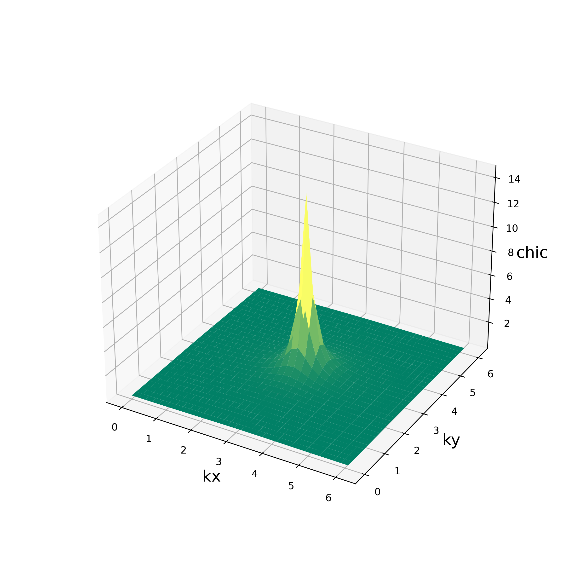
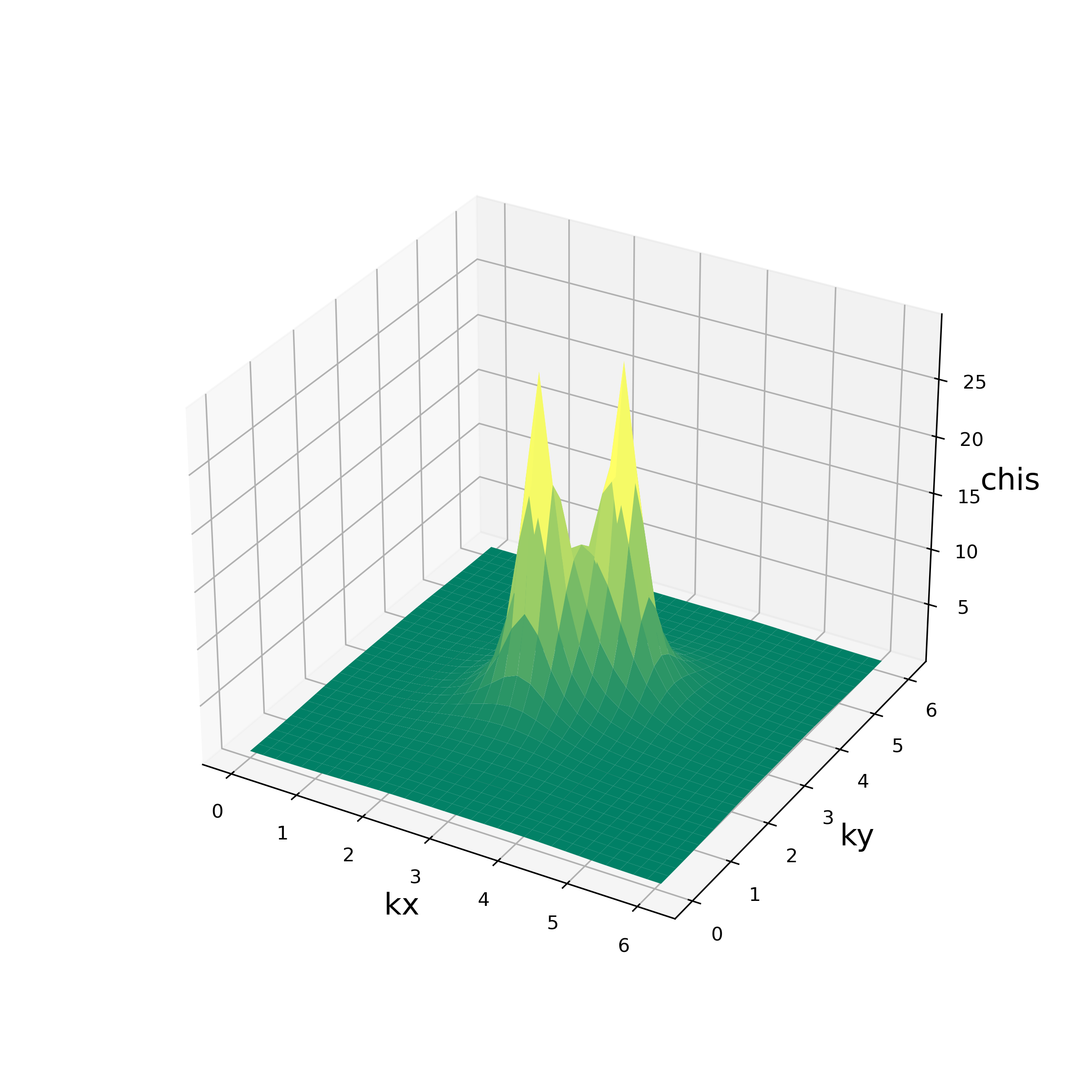
The script reads output/chi0q.npz and output/chiq.npz, and writes the values of
the charge susceptibility \(\chi_c(\vec{q})\)
and the spin susceptibility \(\chi_s(\vec{q})\)
at Matsubara frequency \({\rm i}\omega_m=0\)
for each \(\vec{q}\)
to the standard output.
It also produces the figures of these quantities in PNG format shown as below: