2.2. Kitaev cluster (finite temperatures)

In this subsection, we will examine the convergence of the sampling in the TPQ method. Here, we study a 12 site cluster of a typical magnetically frustrated magnet, the Kitaev model, whose heat capacity shows non-trivial temperature dependence.

The Kitaev model is a kind of the Ising model with bond-orientation dependent Ising interactions as follows:

(2.4)\[H = K \sum_{\gamma=x,y,z}\sum_{\langle i,j\rangle_\gamma}S_{i}^{\gamma} S_{j}^{\gamma},\]

where the index \(\gamma=x,y,z\) specifies the bond direction of the nearest-neighbor site pair \(\langle i,j\rangle_\gamma\).

2.2.1. Lattice structure and eigen states of the Kitaev cluster

A 12 site cluster of the Kitaev model is generated by the following standard input file (samples/tutorial_2.2/stan1.in):

W = 2
L = 3
model = "SpinGC"
method = "CG"
lattice = "Honeycomb"
J0x = -1.0
J0y =  0.0
J0z =  0.0
J1x =  0.0
J1y = -1.0
J1z =  0.0
J2x =  0.0
J2y =  0.0
J2z = -1.0
2S=1
exct = 8

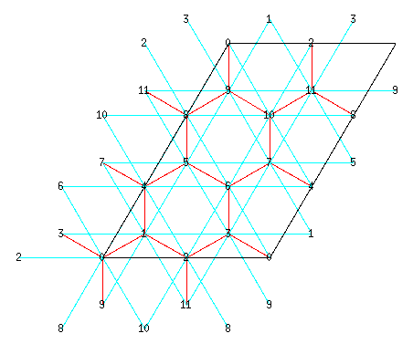
You can visualize the cluster by plotting lattice.gp as shown in the figure below. Here the \(x\) bond (\(\langle i,j\rangle_x\)) connects, for example, the 0th and 1st sites (\(i=0, j=1\)), while the \(y\) bond (\(\langle i,j\rangle_y\)) connects, for example, the 1st and 2nd sites (\(i=1, j=2\)). The :math: z bond (\(\langle i,j\rangle_z\)) connects the 1st and 4th sites for example (\(i=1, j=4\)).

By using the above standard input, we will obtain zvo_energy.dat in your output directory:

State 0
 Energy  -2.4500706750607750
 Doublon  0.0000000000000000
 Sz  0.0000000000333962

State 1
 Energy  -2.4500706750607750
 Doublon  0.0000000000000000
 Sz  -0.0000000000081852

State 2
 Energy  -2.4500706750607804
 Doublon  0.0000000000000000
 Sz  -0.0000000000025177

State 3
 Energy  -2.4500706750607777
 Doublon  0.0000000000000000
 Sz  -0.0000000000018603

State 4
 Energy  -2.3427788601414870
 Doublon  0.0000000000000000
 Sz  0.0000000000982415

State 5
 Energy  -2.3427788601414870
 Doublon  0.0000000000000000
 Sz  -0.0000000000217449

State 6
 Energy  -2.3427788601414830
 Doublon  0.0000000000000000
 Sz  -0.0000000000488295

State 7
 Energy  -2.3427788601414847
 Doublon  0.0000000000000000
 Sz  0.0000000001057668

State 8
 Energy  -2.3237385032276898
 Doublon  0.0000000000000000
 Sz  -0.0647000851410590

State 9
 Energy  -2.3237385032277440
 Doublon  0.0000000000000000
 Sz  0.4412235001577003

2.2.2. Convergence of the microcanonical TPQ

Then, we will examine the convergence of the microcanonical TPQ (mTPQ) method introduced by S. Sugiura and A. Shimizu, which is implemented in H \(\Phi\) for method = “TPQ”.

By using the following standard input file, you can generate 64 mTPQ samples (samples/tutorial_2.2/stan2a.in):

W = 2
L = 3
model = "SpinGC"
method = "TPQ"
lattice = "Honeycomb"
J0x = -1.0
J0y =  0.0
J0z =  0.0
J1x =  0.0
J1y = -1.0
J1z =  0.0
J2x =  0.0
J2y =  0.0
J2z = -1.0
2S=1
Lanczos_max = 3000
LargeValue = 4.0
NumAve = 64

Here, you may use larger Lanczos_max and LargeValue than those in the default setting.

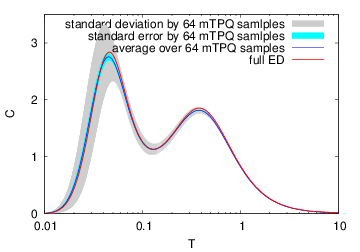
Then, you can obtain the above temperature dependence of the heat capacity. The average of C over the 64 mTPQ samples is shown by the blue curve while C obtained by the full diagonalization is shown by the red curve. The grey belt shows the standard deviation \(\sqrt{\sigma^2}\), and the cyan belt shows the standard error \(\sigma_E = \sqrt{\sigma^2/N_{\rm sample}}\), where \(N_{\rm sample}\) is the sample size (\(N_{\rm sample}=64\)). Although the systematic errors in the estimation of temperatures exist in the mTPQ formalism, the exact hat capacity (the red curve in the above figure) is within the random sample distribution (estimated by \(\sqrt{\sigma^2}\) and shown by the grey belt).

For obtaining the results by the full diagonalization, please use the following input file ((samples/tutorial_2.2/stan2b.in))

W=2
L=3
model = "SpinGC"
method = "fulldiag"
lattice = "Honeycomb"
J0x = -1.0
J0y = 0.0
J0z = 0.0
J1x = 0.0
J1y = -1.0
J1z = 0.0
J2x = 0.0
J2y = 0.0
J2z = -1.0
2S=1

Note that it takes several minute because the dimension of matrix is large (dimension is 4900 ). As in the Heisenberg chain, by using the python script ((``samples/tutorial_2.2/Finite.py``)), you can obtain the temperature dependence of the energy and the specific heat.