2.1. Heisenberg chain (finite temperatures)
Here, we study the finite-temperature properties of spin 1/2 Heisenberg model on the chain.
The input file (samples/tutorial_2.1/stan1.in) for 12-site Heisenberg model is as follows:
L  = 12
J  = 1
2S = 1
model   = "SpinGC"
method  = "cTPQ"
lattice = "chain"
lanczos_max = 2000
LargeValue  = 50
NumAve      = 10
You can execute HPhi as follows
HPhi -s stan1.in
2.1.1. Full diagonalization
After executing the full diagonalization, all the eigenvalues are output in output/Eiegenvalue.dat. By using the python script (samples/tutorial_2.1/Finite.py), you can obtain the temperature dependence of the energy and the specific heat.
You can execute Finite.py as follows
python3 Finite.py
Then, you can obtain FullDiag.dat as follows
0.000100  -5.3873909174000003    0.0000000000000000
0.000150  -5.3873909174000003    0.0000000000000000
0.000200  -5.3873909174000003    0.0000000000000000
0.000250  -5.3873909174000003    0.0000000000000000
0.000300  -5.3873909174000003    0.0000000000000000
The 1st row represents temperature, 2nd row represents the energy, and the 3rd row represents the specific heat defined by \(C=(\langle E^2 \rangle-\langle E \rangle^2)/T^2\).
2.1.2. Micro-canonical TPQ (mTPQ) method (Sz=0)
By selecting method as “TPQ”, you can perform the finite-temperature calculations using the mTPQ method.
The input file (samples/tutorial_2.1/stan2.in) for 12-site Heisenberg model is as follows:
L       = 12
model   = "Spin"
method  = "TPQ"
lattice = "chain"
J = 1
2Sz = 0
2S  = 1
After performing the TPQ calculations, results are output in output/SS_rand*.dat. By using the python script (samples/tutorial_2.1/AveSSrand.py), you can obtain the temperature dependence of physical quantities such as the energy and the specific heat.
Then, you can obtain ave_TPQ.dat as follows
# temperature T    err of T  Energy E    error of E  specific heat C  err of C
30.17747           0.02022   -0.35489    0.04044     0.00264          8.1126-05
15.10875           0.01016   -0.43500    0.04065     0.01068          0.0003182
10.08598           0.00681   -0.51592    0.04086     0.02423          0.0007030
7.574693           0.00513   -0.59754    0.04106     0.04335          0.0012311
6.067978           0.00412   -0.67978    0.04123     0.06808          0.0019053
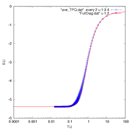
Using gnuplot, you can directly compare the two results
plot "FullDiag.dat" u 1:2 w l,"ave_TPQ.dat" u 1:3:4 w e
You can see the following output image.
2.1.3. mTPQ method (susceptibility)
By using the mTPQ method, it is also possible to calculate the spin susceptibility by performing the calculations for all Sz sectors.
The input file (samples/tutorial_2.1/stan3.in) for 12-site Heisenberg model is as follows:
L       = 12
model   = "SpinGC"
method  = "TPQ"
lattice = "chain"
J = 1
2S  = 1
Here, note that “model = Spin” is changed to “model = SpinGC” and “Sz = 0” is omitted.
After performing the TPQ calculations, temperature dependence of several physical quantities such as number of particel N and total Sz are output in output/Flct_rand*.dat. By using the python script (samples/tutorial_2.1/AveFlct.py), you can obtain the temperature dependence of physical quantities such as the energy and the spin susceptibility \(\chi\). Note that \(\chi\) is defined as
Then, you can obtain ave_Flct.dat as follows
# temperature T    err of T  m_z         error of m_z susceptibility chi  err of chi
13.5876            0.00695   -0.00688    0.00955      0.21243             0.00184
6.83615            0.00373   -0.00783    0.01067      0.40632             0.00414
4.58603            0.00278   -0.00894    0.01251      0.58234             0.00694
3.46113            0.00239   -0.01023    0.01474      0.74129             0.01021
2.78624            0.00220   -0.01171    0.01713      0.88407             0.01383
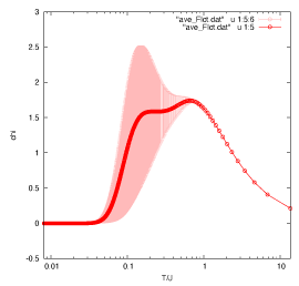
Using gnuplot, you can see the temperature dependence of \(\chi\)
se log x
se colors classic
se xlabel "T/J"
se ylabel "chi"
plot    "ave_Flct.dat"   u 1:5:6 w e lc rgb "#FFBBBB" ps 1 pt 6,\
        "ave_Flct.dat"   u 1:5 w lp lt 1 ps 1 pt 6
You can see the following output image.
2.1.4. Canonical TPQ (cTPQ) method (Advanced)
In the cTPQ method, we generate the kth TPQ state as
where \(n_{\rm max}\) represents the order of the Taylor expansion and \(\Delta\tau\) represents increment of the imaginary-time evolution. An advantage of the cTPQ method is the inverse temperatures do not depend on the initial states \(\ket{\Phi_{\rm rand}}\). Because of this feature, it is possible to estimate the errors originating from fluctuations of the initial states without ambiguity using the bootstarp method.
A input file (samples/tutorial_2.1/stan4.in) for 12-site Heisenberg model is as follows:
L  = 12
J  = 1
2S = 1
model   = "SpinGC"
method  = "cTPQ"
lattice = "chain"
lanczos_max = 2000
LargeValue  = 50
NumAve      = 10
The increment of the imaginary-time evolution \(\Delta\tau\) is given by \(\Delta\tau=1/{\rm LargeValue }=1/50=0.02\). The default value of \(n_{\rm max}=10\) is used in this calculation. Please note that this cTPQ calculation takes 2-3 minutes.
After the calculation, by executing sh Aft_cTPQ.sh,
you can estimate the average values and errors by using the bootstrap method.
In this example, we choose 10 samples from 10 samples with allowing
duplications for 5 times in the bootstrap sampling.
In BS_MaxBS5.dat, the following physical quantities are output:
T E E_err C C_err S S_err Sz Sz_err chi_Sz chi_Sz_err Z Z_err k
where
T: temperature (\(T=1/\beta=1/(k\Delta\tau)\)),E: average value of energy,E_err: error of energy,C: average value of specific heat,C_err: error of specific heat,S: average value of entropy,S_err: error of entropy,Sz: average value of Sz,Sz_err: error of Sz,chi_Sz: average value of chi_Sz,chi_Sz_err: error of chi_Sz,Z: average value of norm the wave function,Z_err: error of norm of the wave function, andk: number of the cTPQ state.
For example, you can see the temperature dependence of the specific heat as:
se log x
se colors classic
se xlabel "T/J"
se ylabel "C"
plot    "BS_MaxBS5.dat"  u 1:4:5 w e lt 1 ps 1 pt 6
We note that Ext_BS_MaxBS5.dat is a file with several temperatures omitted from
BS_MaxBS5.dat for clarity. To see overall temperature dependence, it is better to
plot Ext_BS_MaxBS5.dat.
More advanced exercise:
By increasing NumAve (e.g. NumAve=100),
please examine how the error bars of the physical quantities decrease.