1.5. J1-J2 Heisenberg model
Here, we solve the \(J_{1}-J_{2}\) Heisenberg model on the square lattice, which is a canonical example of the frustrated magnets. Its Hamiltonian is defined as
where \(J_{1}\) (\(J_{2}\)) represents the nearest (next-nearest) neighbor interactions.
An input file (samples/tutorial_1.5/stan1.in) for treating \(J_{1}-J_{2}\) Heisenberg model is given as
model = "Spin"
method = "CG"
lattice = "square"
L = 4
W = 4
J = 1
J' = 1
2S = 1
2Sz = 0
exct = 4
Here, J (J’) represents \(J_{1}\) (\(J_{2}\)).
1.5.1. Calculations of spin structure factors for ground state
First, we calculate the spin structure factors, which are defined as
To calculate \(S({\bf q})\), it is necessary to prepare
a proper input file for two-body Green functions.
By using a python script MakeGreen.py (samples/tutorial_1.5/MakeGreen.py),
you can generate greentwo.def for calculating \(S({\bf q})\).
To use MakeGreen.py , an input file for specifying lattice geometry (input.txt, samples/tutorial_1.5/input.txt) is necessary,
whose form is given as follows
Lx 4
Ly 4
Lz 1
orb_num 1
Here, Lx (orb_num) represents the length of the x direction (number of orbitals).
By using a python script CalcSq.py (samples/tutorial_1.5/CalcSq.py),
you can calculate \(S({\bf q})\) from output/zvo_cisajscktalt_eigen0.dat.
- Procedure for calculating and visualizing \(S({\bf q})\) is given as follows ::
HPhi -sdry stan.in
python3 MakeGreen.py (input.txt is necessary)
HPhi -e namelist.def
python3 CalcSq.py (input.txt is necessary)
You can obtain Sq_eigen0.dat !!
splot “Sq_eigen0.dat” u 1:2:3 (using gnuplot)
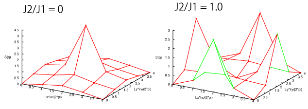
Following the procedure, please see how \(S({\bf q})\) changes by changing J’. As an example, we show \(S({\bf q})\) for J1/J2=0 and 1 below.
1.5.2. Calculations of spin structure factors for excited states
By changing exct in stan.in, you can obtain several excited states. For those excited states, by changing max_num=1 in CalcSq.py as, for example, max_num=4, you can obtain \(S({\bf q})\) for the excited states. As a practice for editing file, please try to edit CalcSq.py manually (open CalcSq.py, finding variable max_num =1, and changing max_num = 4).
Please see how \(S({\bf q})\) in the excited states changes by changing J’. For example, please check what is the nature of the first excited state J’=0,0.5, and 1.