3.2. Example for moller calculation with HPhi

What’s this sample?

This is an example of moller with HPhi, which is an open-source software package for performing the exact diagonalization method for quantum many-body problems. In this example, we will calculate the system size dependence of the excitation gap \(\Delta\) of the \(S=1/2\) (2S_1 directory) and \(S=1\) (2S_2) antiferromagnetic Heisenberg chain under the periodic boundary condition. By using moller, calculations with different system sizes are performed in parallel. This is corresponding to section 1.4 of HPhi’s official tutorial.

Preparation

Make sure that moller (HTP-tools) package and HPhi are installed. In this tutorial, the calculation will be performed using the supercomputer system ohtaka at ISSP.

How to run

1. Prepare dataset

   Run the script make_inputs.sh enclosed within this package.

   $ bash ./make_inputs.sh
   

   Working directories L_8, L_10, …, L_24 (up to L_18 for 2S_2)) will be generated. A list of the directories is written to a file list.dat. Additionally, a shell script, extract_gap.sh, to gather energy gaps from working directories is generated.

2. Generate job script using moller

   Generate a job script from the job description file using moller, and store the script as a file named job.sh.

   $ moller -o job.sh input.yaml
   

3. Run batch job

   Submit a batch job with the job list as an argument.

   $ sbatch job.sh list.dat
   

4. Check status

   The status of task execution will be summarized by moller_status program.

   $ moller_status input.yaml list.dat
   

5. Gather results

   Once the calculation finishes, gather energy gaps from jobs as

   $ bash extract_gap.sh
   

   This script writes pairs of the length \(L\) and the gap \(\Delta\) into a text file, gap.dat.

   To visualize the results, a Gnuplot file gap.plt is available. In this file, the obtained gap data are fitted by the expected curves,

   (3.1)\[\Delta(L; S=1/2) = \Delta_\infty + A/L\]

   and

   (3.2)\[\Delta(L; S=1) = \Delta_\infty + B\exp(-CL).\]

   The result is plotted as follows:

   $ gnuplot --persist gap.plt
   

   

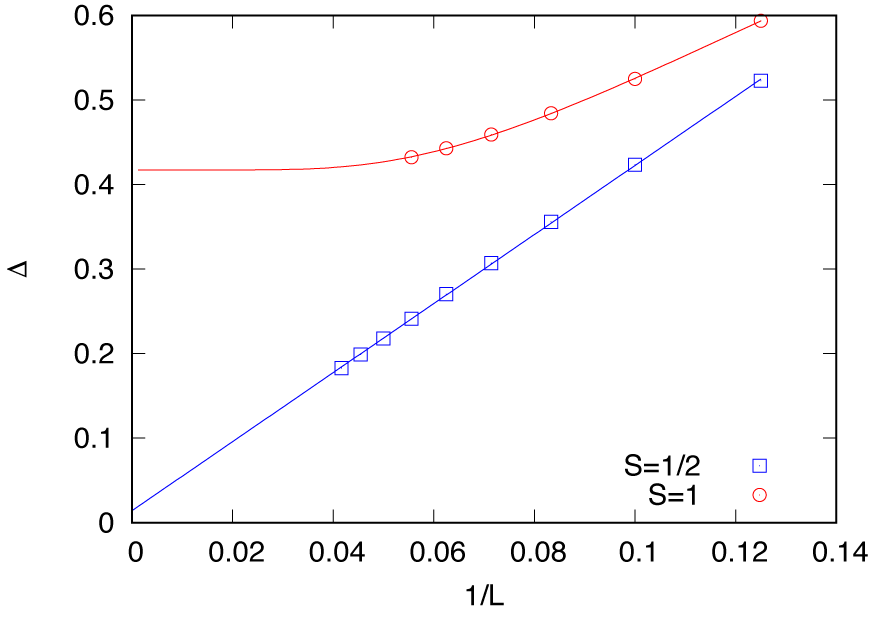
   Fig. 3.3 Finite size effect of spin gap

   Note that the logarithmic correction causes the spin gap for \(S=1/2\) to remain finite. On the other hand, for \(S=1\), the extrapolated value \(\Delta_\infty = 0.417(1)\) is consistent with the previous results, e.g., \(\Delta_\infty = 0.41048(6)\) by QMC (Todo and Kato, PRL 87, 047203 (2001)).