Search by replica exchange Monte Carlo#
This tutorial describes how to solve the minimization problem of the Himmelblau function by using the replica exchange Monte Carlo method (RXMC).
Sample files#
Sample files are available from sample/analytical/exchange.
This directory includes the following files:
input.tomlThe input file of odatse
do.shScript for running this tutorial
Input files#
This subsection describes the input file. For details, see the “Input file” chapter and Replica exchange Monte Carlo exchange.
[base]
dimension = 2
output_dir = "output"

[solver]
name = "analytical"
function_name = "himmelblau"

[algorithm]
name = "exchange"
seed = 12345

[algorithm.param]
min_list = [-6.0, -6.0]
max_list = [6.0, 6.0]
step_list = [0.3, 0.3]

[algorithm.exchange]
Tmin = 0.01
Tmax = 100.0
numsteps = 10000
numsteps_exchange = 100
nreplica_per_proc = 20
In the following, we will briefly describe this input file. For details, see the manual of Replica exchange Monte Carlo exchange.
The contents of the [base] and [solver] sections are the same as those for the search by the Nelder-Mead method (minsearch).
[algorithm] section specifies the algorithm to use and its settings.
nameis the name of the algorithm you want to use. In this tutorial we will use RXMC, so specifyexchange.seedis the seed that a pseudo-random number generator uses.
[algorithm.param] section sets the parameter space to be explored.
min_listis a lower bound andmax_listis an upper bound.step_listis the step length of one Monte Carlo update (standard deviation of the Gaussian distribution).
[algorithm.exchange] section sets the hyperparameters for RXMC.
numstepsis the number of Monte Carlo steps.numsteps_exchangeis the number of steps between temperature exchanges.Tmin,Tmaxare the minimum and the maximum of temperature, respectively.When
Tlogspaceistrue, the temperature points are distributed uniformly in the logarithmic space.nreplica_per_procspecifies the number of replicas that one MPI process handles.
Calculation#
First, move to the folder where the sample file is located. (Hereinafter, it is assumed that you are in the root directory of ODAT-SE.)
$ cd sample/analytical/exchange
Then, run the main program. It will take a few seconds on a normal PC.
$ mpiexec -np 4 odatse input.toml | tee log.txt
Here, the calculation is performed using MPI parallel with 4 processes.
If you are using Open MPI and you request more processes than the number of cores, you need to add the --oversubscribe option to the mpiexec command.
When executed, a folder for each MPI rank will be created under output directory, and a trial.txt file containing the parameters evaluated in each Monte Carlo step and the value of the objective function, and a result.txt file containing the parameters actually adopted will be created.
These files have the same format: the first two columns are time (step) and the index of walker in the process, the third is the temperature, the fourth column is the value of the objective function, and the fifth and subsequent columns are the parameters.
# step walker T fx x1 x2
0 0 0.01 187.94429125133564 5.155393113805774 -2.203493345018569
0 1 0.01123654800138751 3.179380982615041 -3.7929742598748666 -3.5452766573635235
0 2 0.012626001098748564 108.25464277273859 0.8127003489802398 1.1465364357510186
0 3 0.014187266741165962 483.84183395038843 5.57417423682746 1.8381251624588506
0 4 0.01594159037455999 0.43633134370869153 2.9868796504069426 1.8428384502208246
0 5 0.01791284454622004 719.7992581349758 2.972577711255287 5.535680832873856
0 6 0.020127853758499396 452.4691017123836 -5.899340424701358 -4.722667479627368
0 7 0.022616759492228647 45.5355817998709 -2.4155554347674215 1.8769341969872393
0 8 0.025413430367026365 330.7972369561986 3.717750630491217 4.466110964691396
0 9 0.028555923019901074 552.0479484091458 5.575771168463163 2.684224163039442
0 10 0.032086999973704504 32.20027165958588 1.7097039347500953 2.609443449748964
...
best_result.txt is filled with information about the parameter with the optimal objective function, the rank from which it was obtained, and the Monte Carlo step.
nprocs = 80
rank = 2
step = 1632
walker = 9
fx = 3.618846176852812e-06
x1 = -2.8054241034292455
x2 = 3.13143739585623
nprocs in the first line denotes the total number of replicas (the number of MPI processes × nreplica_per_proc; 4 × 20 = 80 in this example).
Note that the Himmelblau function has four global minima; in this run, the solution near one of them, \((-2.805, 3.131)\), is obtained.
In ODAT-SE, one replica holds samples at different temperatures because of the temperature exchanges. The result.txt in each rank folder records the data sampled by each replica.
The data reorganized for each temperature point is written to output/result_T%.txt, where % is the index of the temperature point.
The first column is the step, the second column is the global walker (replica) index, the third column is the value of the objective function, and the fourth and subsequent columns are the parameters.
Example:
# T = 0.014187266741165962
0 3 483.84183395038843 5.57417423682746 1.8381251624588506
1 3 376.63669411179063 5.315947017297935 2.006168750367261
2 3 376.63669411179063 5.315947017297935 2.006168750367261
3 3 376.63669411179063 5.315947017297935 2.006168750367261
4 3 376.63669411179063 5.315947017297935 2.006168750367261
5 3 254.81573883689714 5.04750307814821 1.483720563950596
...
Visualization#
By plotting output/result_T%.txt, you can estimate regions where the parameters with small function values are located.
By executing the following command, the two-dimensional plots res_T%.png will be generated.
$ python3 ../plot_himmel.py --xcol=3 --ycol=4 --skip=20 --format="o" --output=output/res_T0.png output/result_T0.txt
Looking at the resulting diagram, we can see that the samples are concentrated near the minima of f(x). By changing the index of the temperature, the sampling points scatter over the region at high temperature, while they tend to concentrate on the minima at low temperature.
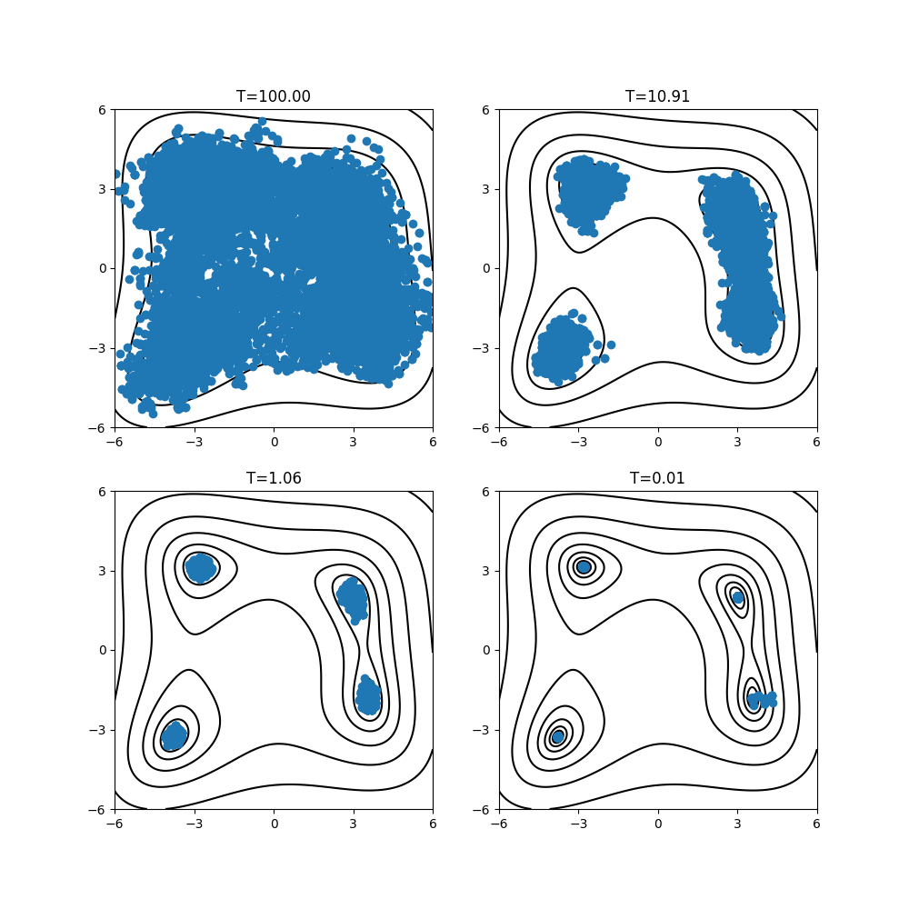
Fig. 7 Distribution of sampling points on two-dimensional parameter space at \(T=\{35.02, 3.40, 0.33, 0.01\}\).#
See also
Post-processing tools are available for analyzing the calculation results,
such as odatse_separateT, which splits Monte Carlo log files by temperature point.
See Post-Processing Tools for details.