3.4. DSQSS/DLA による正方格子上ハードコアボソン系の粒子数計算

このチュートリアルでは, 大きさ \(8\times8\) の正方格子上の, \(V/t=3, \beta t = 10\) というパラメータを持つハードコアボーズハバード模型について, 化学ポテンシャル \(\mu\) を \(-4.0\) から \(14.0\) まで動かして計算を行い, 粒子数密度の変化を計算します.

次に示すのは, 入力ファイルの生成と本計算を自動で行い, 粒子数密度の化学ポテンシャル依存性をファイルに書き出すスクリプトです(sample/dla/03_bosesquare/exec.py).

import subprocess

from dsqss.dla_pre import dla_pre
from dsqss.result import Results

V = 3
L = [8, 8]
beta = 10.0

lattice = {"lattice": "hypercubic", "dim": 2, "L": L}
hamiltonian = {"model": "boson", "t": 1, "V": V, "M": 1}
parameter = {"beta": beta, "nset": 4, "ntherm": 100, "ndecor": 100,
             "nmcs": 100, "wvfile": "wv.xml", "dispfile": "disp.xml"}

name = "amzu"
mus = [-4.0, -2.0, 0.0, 2.0, 2.5, 3.0, 6.0, 9.0, 9.5, 10.0, 12.0, 14.0]

output = open("{}.dat".format(name), "w")
for i, mu in enumerate(mus):
    ofile = "res_{}.dat".format(i)
    pfile = "param_{}.in".format(i)
    sfoutfile = "sf_{}.dat".format(i)
    cfoutfile = "cf_{}.dat".format(i)
    ckoutfile = "ck_{}.dat".format(i)

    hamiltonian["mu"] = mu
    parameter["outfile"] = ofile
    parameter["sfoutfile"] = sfoutfile
    parameter["cfoutfile"] = cfoutfile
    parameter["ckoutfile"] = ckoutfile
    dla_pre(
        {"parameter": parameter, "hamiltonian": hamiltonian, "lattice": lattice}, pfile
    )
    cmd = ["dla", pfile]
    subprocess.call(cmd)
    res = Results(ofile)
    output.write("{} {}\n".format(mu, res.to_str(name)))
output.close()

このPython スクリプトを実行すると

$ python exec.py

化学ポテンシャルごとに密度の期待値と統計誤差が amzu.dat に行ごとにスペース区切りで書き出されます. このファイルをGnuplot などで図示すると(図 3.2). \(\mu=6\) 付近では密度プラトーが観測されます. ここでは近接サイト間の反発によりチェッカーボード固体相になっています.

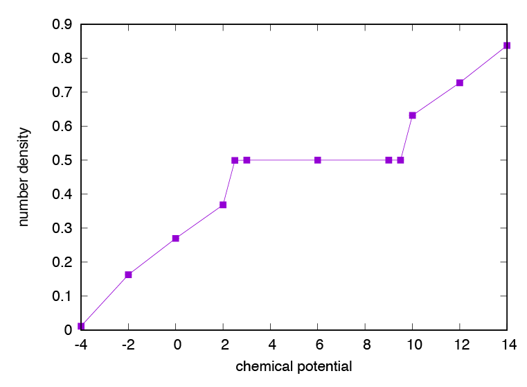
図 3.2 正方格子上のボースハバード模型における密度の化学ポテンシャル依存性.