3.3. DSQSS/DLA によるスピン鎖の帯磁率計算

このチュートリアルでは, 局在スピンの大きさが \(S=1/2, 1\) である2種類の 反強磁性ハイゼンベルグ鎖 (\(J=-1, L=30\)) において, 温度 \(T\) を \(0.05\) から \(2.0\) まで動かしたときの 帯磁率変化を計算します.

次に示すのは, 温度やスピンの大きさを変えながら入力ファイルの生成と本計算を自動で行い, 帯磁率の温度依存性をファイルに書き出す Pythonスクリプトです(sample/dla/02_spinchain/exec.py).

import subprocess

from dsqss.dla_pre import dla_pre
from dsqss.result import Results

L = 30

lattice = {"lattice": "hypercubic", "dim": 1, "L": L}
hamiltonian = {"model": "spin", "Jz": -1, "Jxy": -1}
parameter = {"nset": 5, "ntherm": 1000, "ndecor": 1000, "nmcs": 1000,
             "wvfile": "wv.xml", "dispfile": "disp.xml"}

name = "xmzu"
Ms = [1, 2]
Ts = [0.05, 0.1, 0.2, 0.3, 0.4, 0.5, 0.6, 0.7, 0.8, 0.9, 1.0, 1.25, 1.5, 1.75, 2.0]

for M in Ms:
    output = open("{0}_{1}.dat".format(name, M), "w")
    for i, T in enumerate(Ts):
        ofile = "res_{}_{}.dat".format(M, i)
        pfile = "param_{}_{}.in".format(M, i)
        sfoutfile = "sf_{}_{}.dat".format(M, i)
        cfoutfile = "cf_{}_{}.dat".format(M, i)
        ckoutfile = "ck_{}_{}.dat".format(M, i)
        hamiltonian["M"] = M
        parameter["beta"] = 1.0 / T
        parameter["outfile"] = ofile
        parameter["sfoutfile"] = sfoutfile
        parameter["cfoutfile"] = cfoutfile
        parameter["ckoutfile"] = ckoutfile
        dla_pre(
            {"parameter": parameter, "hamiltonian": hamiltonian, "lattice": lattice},
            pfile,
        )
        cmd = ["dla", "param_{0}_{1}.in".format(M, i)]
        subprocess.call(cmd)
        res = Results(ofile)
        output.write("{} {}\n".format(T, res.to_str(name)))
    output.close()

このPython スクリプトを実行すると

$ python exec.py

\(S=1/2\) の結果が xmzu_1.dat に, \(S=1\) の結果が xmzu_2.dat にそれぞれ書き出されます. ファイルの各行には温度, 帯磁率の期待値, 帯磁率の統計誤差が順に書き出されます. この2つのファイルをGnuplot などで図示すると(図 3.1), スピンの大きさによって, スピンギャップの有無が異なり, その結果として絶対零度付近での帯磁率の振る舞いが異なってくることがわかります.

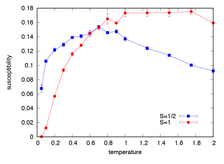
図 3.1 反強磁性ハイゼンベルグスピン鎖の帯磁率の温度依存性. 青が \(S=1/2\) で 赤が \(S=1\) の結果.