Replica Exchange Monte Carlo search with limitation

This tutorial describes the constraint expression function that can be set in the [runner.limitation] section. As an example, the replica exchange Monte Carlo method is applied to the calculation of Himmelblau with constraints.

Sample files location

Sample files are available in the sample/analytical/limitation directory. This directory contains the following files.

• ref.txt

  File to check if the calculation is executed correctly (answer to obtain by performing this tutorial).

• input.toml

  Input file for the main program.

• do.sh

  Script prepared to calculate this tutorial at once.

In the following, we will explain these files, and then introduce the actual calculation results.

Input files

The following input.toml is an input file for the main program.

[base]
dimension = 2
output_dir = "output"

[algorithm]
name = "exchange"
seed = 12345

[algorithm.param]
max_list = [6.0, 6.0]
min_list = [-6.0, -6.0]
unit_list = [0.3, 0.3]

[algorithm.exchange]
Tmin = 1.0
Tmax = 100000.0
numsteps = 10000
numsteps_exchange = 100

[solver]
name = "analytical"
function_name = "himmelblau"

[runner]
[runner.limitation]
co_a = [[1, -1],[1, 1]]
co_b = [[0], [-1]]

[base] section is the parameter of the main program. dimension is the number of variables to be optimized, and in this case, it is 2.

[algorithm] section is the section to set the search algorithm. name is the name of the search algorithm. In this case, specify "exchange" for the replica exchange Monte Carlo method. seed is the seed given to the pseudo-random number generator.

[algorithm.param] sub-section specifies the range of parameters to be optimized. min_list indicates the minimum value, and max_list indicates the maximum value.

[algorithm.exchange] sub-section specifies the hyperparameters of the replica exchange Monte Carlo method.

• numstep is the number of Monte Carlo updates.

• numsteps_exchange specifies the number of times to attempt temperature exchange.

• Tmin and Tmax are the lower and upper limits of the temperature, respectively.

• If Tlogspace is true, the temperature is divided equally in log space. This option is not specified in this input.toml because the default value is true.

[solver] section specifies the solver used internally in the main program. In this case, the analytical solver is specified. The analytical solver sets the function using the function_name parameter, and in this case, the Himmelblau function is specified.

[runner] section has a sub-section [runner.limitation], and in this section, the constraint expression is set. In the current version, the constraint expression is defined as \(Ax+b>0\) where \(x\) is \(N\) dimensional input parameter, \(A\) is a \(M \times N\) matrix, and \(b\) is a \(M\) dimensional vector. \(A\) and \(b\) are set by co_a and co_b, respectively. For details, see the [limitation] section in the input file in the manual.

In this case, the following constraint is imposed:

\[\begin{split}x_{1} − x_{2} > 0\\ x_{1} + x_{2} − 1 > 0\end{split}\]

Calculation

First, move to the folder where the sample file is located (assuming that you are directly under the directory where you downloaded this software).

cd sample/analytical/limitation

Then, execute the main program as follows (the calculation time will end in about 20 seconds on a normal PC).

mpiexec -np 10 python3 ../../../src/py2dmat_main.py input.toml | tee log.txt

In this case, a calculation with 10 MPI parallel processes is performed. (When using OpenMPI, if the number of processes to be used is greater than the number of available cores, add the --oversubscribed option to the mpiexec command.) After executed, the output folder is generated, and in it, a subfolder for each rank is created. Each subfolder contains the results of the calculation. trial.txt file, which contains the parameters and objective function values evaluated at each Monte Carlo step, and result.txt file, which contains the parameters actually adopted, are created. Both files have the same format, with the first two columns being the step number and the walker number within the process, the next being the temperature, the third being the value of the objective function, and the fourth and subsequent being the parameters. The following is the beginning of the output/0/result.txt file:

# step walker T fx x1 x2
0 0 1.0 187.94429125133564 5.155393113805774 -2.203493345018569
1 0 1.0 148.23606736778044 4.9995614992887525 -2.370212436322816
2 0 1.0 148.23606736778044 4.9995614992887525 -2.370212436322816
3 0 1.0 148.23606736778044 4.9995614992887525 -2.370212436322816

Finally, the best parameter and the rank and Monte Carlo step at which the objective function is minimized are written to output/best_result.txt.

nprocs = 10
rank = 2
step = 4523
walker = 0
fx = 0.00010188398524402734
x1 = 3.584944906595298
x2 = -1.8506985826548874

do.sh is available as a script to calculate all at once. Additionally, in do.sh, the difference between best_result.txt and ref.txt is also compared.

#!/bin/bash
mpiexec -np 10 --oversubscribe python3 ../../../src/py2dmat_main.py input.toml

echo diff output/best_result.txt ref.txt
res=0
diff output/best_result.txt ref.txt || res=$?
if [ $res -eq 0 ]; then
  echo TEST PASS
  true
else
  echo TEST FAILED: best_result.txt and ref.txt differ
  false
fi

Visualization of the calculation result

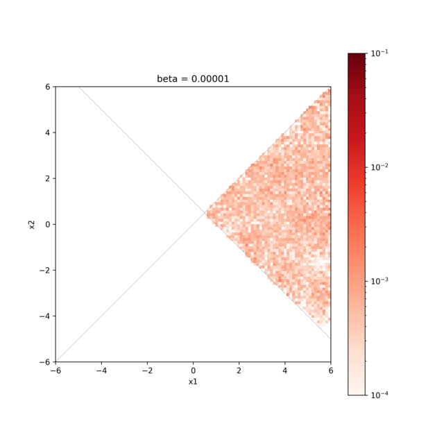
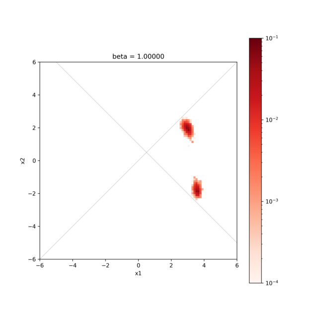
By visualizing the result.txt file, we can confirm that the search is only for coordinates that satisfy the constraint expression. hist2d_limitation_sample.py is prepared to visualize the 2D parameter space. This generates a histogram of the posterior probability distribution in the <execution date>_histogram folder. The histogram is generated using the data obtained by discarding the first 1000 steps of the search as a burn-in period.

python3 hist2d_limitation_sample.py -p 10 -i input.toml -b 0.1

The figure shows the posterior probability distribution and the two lines \(x_{1} − x_{2} = 0, x_{1} + x_{2} − 1 = 0\), and it is confirmed that the search is only for the range where \(x_{1} − x_{2} > 0, x_{1} + x_{2} − 1 > 0\).