Optimization by population annealing

This tutorial subscribes how to estimate atomic positions from the experimental diffraction data by using the population annealing Monte Carlo method (PAMC).

Sample files

Sample files are available from sample/sim-trhepd-rheed/single_beam/pamc . This directory includes the following files:

• bulk.txt

  The input file of bulk.exe

• experiment.txt , template.txt

  Reference files for the main program

• ref.txt

  Solution file for checking whether the calucation successes or not (reference for fx.txt)

• input.toml

  The input file of py2dmat

• prepare.sh , do.sh

  Script files for running this tutorial

In the following, we will subscribe these files and then show the result.

Reference files

This tutorial uses reference files, template.txt and experiment.txt, which are the same as the previous tutorial (Optimization by Nelder-Mead method) uses.

Input files

This subsection describes the input file. For details, see the manual of bayes. input.toml in the sample directory is shown as the following

[base]
dimension = 2
output_dir = "output"

[algorithm]
name = "pamc"
label_list = ["z1", "z2"]
seed = 12345

[algorithm.param]
min_list = [3.0, 3.0]
max_list = [6.0, 6.0]
unit_list = [0.3, 0.3]

[algorithm.pamc]
numsteps_annealing = 5
bmin = 0.0
bmax = 200.0
Tnum = 21
Tlogspace = false
nreplica_per_proc = 10

[solver]
name = "sim-trhepd-rheed"

[solver.config]
calculated_first_line = 5
calculated_last_line = 74
row_number = 2

[solver.param]
string_list = ["value_01", "value_02" ]
degree_max = 7.0

[solver.reference]
path = "experiment.txt"
first = 1
last = 70

In the following, we will briefly describe this input file. For details, see the manual of Replica exchange Monte Carlo exchange.

• The [base] section describes the settings for a whole calculation.

  • dimension is the number of variables you want to optimize. In this case, specify 2 because it optimizes two variables.

• The [solver] section specifies the solver to use inside the main program and its settings.

  • See the minsearch tutorial.

• The [algorithm] section sets the algorithm to use and its settings.

  • name is the name of the algorithm you want to use, and in this tutorial we will use RXMC, so specify exchange.

  • label_list is a list of label names to be given when outputting the value of value_0x (x = 1,2).

  • seed is the seed that a pseudo-random number generator uses.

  • The [algorithm.param] section sets the parameter space to be explored.

    • min_list is a lower bound and max_list is an upper bound.

    • unit_list is step length in one MC update (deviation of Gaussian)

  • The [algorithm.pamc] section sets the parameters for PAMC.

    • numsteps_annealing is the number of interval steps between temperature decreasing.

    • bmin, bmax are the minimum and the maximum of inversed temperature, respectively.

    • Tnum is the number of (inversed) temperature points.

    • When Tlogspace is true, the temperature points are distributed uniformly in the logarithmic space.

    • nreplica_per_proc is the number of replicas (MC walkers) in one MPI process.

• The [solver] section specifies the solver to use inside the main program and its settings.

  • See the Optimization by Nelder-Mead method tutorial.

Calculation

First, move to the folder where the sample file is located (hereinafter, it is assumed that you are the root directory of 2DMAT).

cd sample/sim-trhepd-rheed/single_beam/pamc

Copy bulk.exe and surf.exe as the tutorial for the direct problem.

cp ../../../../../sim-trhepd-rheed/src/TRHEPD/bulk.exe .
cp ../../../../../sim-trhepd-rheed/src/TRHEPD/surf.exe .

Execute bulk.exe to generate bulkP.b .

./bulk.exe

Then, run the main program (it takes a few secondes)

mpiexec -np 4 python3 ../../../../src/py2dmat_main.py input.toml | tee log.txt

Here, the calculation is performed using MPI parallel with 4 processes. (If you are using Open MPI and you request more processes than you can use, add the --oversubscribed option to the mpiexec command.)

When executed, a folder for each rank will be created, and trial_TXXX.txt files containing the parameters evaluated in each Monte Carlo step and the value of the objective function at each temperature (XXX is the index of points), and result_TXXX.txt files containing the parameters actually adopted will be created. These files are concatnated into result.txt and trial.txt.

These files have the same format: the first two columns are time (step) and the index of walker in the process, the third is the (inversed) temperature, the fourth column is the value of the objective function, and the fifth and subsequent columns are the parameters. The final two columns are the weight of walker (Neal-Jarzynski weight) and the index of the grand ancestor (the replica index at the beginning of the calculation).

# step walker beta fx z1 z2 weight ancestor
0 0 0.0 0.07702743614780189 5.788848278451443 3.949126663745358 1.0 0
0 1 0.0 0.08737730661436376 3.551756435031283 3.6136808356591192 1.0 1
0 2 0.0 0.04954470587051104 4.70317508724506 4.786634108937754 1.0 2
0 3 0.0 0.04671675601156148 5.893543559206865 4.959531290614713 1.0 3
0 4 0.0 0.04142014655238446 5.246719912601735 4.960709612555206 1.0 4

In the case of the sim-trhepd-rheed solver, a subfolder Log%%%%% (%%%%% is the number of MC steps) is created under each working folder, and locking curve information etc. are recorded.

Finally, best_result.txt is filled with information about the parameter with the optimal objective function (R-factor), the rank from which it was obtained, and the Monte Carlo step.

nprocs = 4
rank = 0
step = 71
walker = 5
fx = 0.008186713312593607
z1 = 4.225633749839847
z2 = 5.142666117413409

Finally, fx.txt stores the statistics at each temperature point:

# $1: 1/T
# $2: mean of f(x)
# $3: standard error of f(x)
# $4: number of replicas
# $5: log(Z/Z0)
# $6: acceptance ratio
0.0 0.06428002079611472 0.002703413400677839 40 0.0 0.795
10.0 0.061399304916174735 0.002649424392996749 40 -0.6280819199879947 0.85
20.0 0.05904248889111052 0.0031622711212952034 40 -1.2283060742855603 0.74
30.0 0.04956921148431115 0.0028298565759159633 40 -1.7991035905899855 0.67

The first column is (inversed) temperature, and the second/third ones are the mean and standard error of \(f(x)\), respectively. The fourth column is the number of replicas and the fifth one is the logarithm of the ratio of the partition functions, \(\log(Z_n/Z_0)\), where \(Z_0\) is the partition function at the first temperature. The sixth column is the acceptance ratio of MC updates.

In addition, do.sh is prepared as a script for batch calculation. do.sh also checks the difference between best_result.txt and ref.txt. I will omit the explanation below, but I will post the contents.

sh prepare.sh

./bulk.exe

time mpiexec --oversubscribe -np 4 python3 ../../../../src/py2dmat_main.py input.toml

echo diff output/fx.txt ref.txt
res=0
diff output/fx.txt ref.txt || res=$?
if [ $res -eq 0 ]; then
  echo TEST PASS
  true
else
  echo TEST FAILED: output/fx.txt and ref.txt differ
  false
fi

Visualization

By illustrating result_T.txt, you can estimate regions where the parameters with small R-factor are. In this case, the figure result_fx.pdf and result_T.pdf of the 2D parameter space is created by using the following command. The color of symbols of result_fx.pdf and result_T.pdf mean R-factor and \(\beta\), respectively.

python3 plot_result_2d.py

Looking at the resulting diagram, we can see that the samples are concentrated near (5.25, 4.25) and (4.25, 5.25), and that the R-factor value is small there.

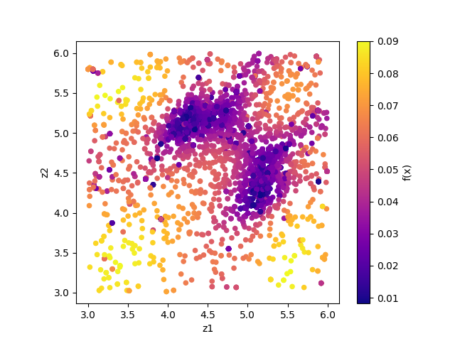
Fig. 5 Sampled parameters and R-factor. The horizontal axes is value_01 and the vertical axes is value_02 .

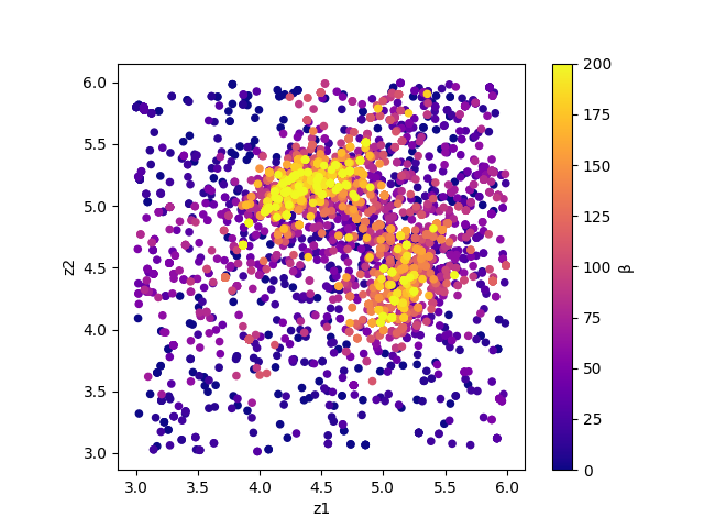
Fig. 6 Sampled parameters and \(\beta\). The horizontal axes is value_01 and the vertical axes is value_02 .

Also, RockingCurve.txt is stored in each subfolder, LogXXX_YYY (XXX is an index of MC step and YYY is an index of a replica in the MPI process). By using this, it is possible to compare with the experimental value according to the procedure of the previous tutorial.