Analytic continuation with the Pade approximation
The Pade approximation is a simple and widely used method for the analytic continuation.
The Pade approximation is based on the assumption that the Green’s function can be approximated by a rational function of the frequency.
The Pade approximation is implemented in the dcore_anacont program.
The common parameters of dcore_anacont is specified in the [post.anacont] block as follows:
[post.anacont]
solver = pade
omega_min = -6.0
omega_max = 6.0
Nomega = 101
show_result = false
save_result = true
solver specifies the method for the analytic continuation.
omega_min, omega_max, and Nomega specify the frequency range and the number of frequency points for the output;
the frequency points are linearly spaced between omega_min and omega_max.
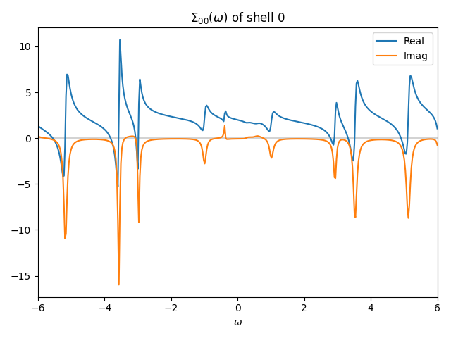
show_result specifies whether the obtained self-energies \(\mathrm{Re}\Sigma_{ij}(\omega)\) and \(\mathrm{Im}\Sigma_{ij}(\omega)\) are displayed on the screen by using Matplotlib.
save_result specifies whether the plots of the obtained self-energies are saved in the work/post directory as sigma_w_{ish}_{iorb}_{jorb}.png,
where ish is the shell index, and iorb and jorb are the orbital indices.
The output directory work/post can be changed by the parameter dir_work in the [post] block.
The parameters for the Pade approximation are specified in the [post.anacont.pade] block as follows:
[post.anacont.pade]
iomega_max = 10000
n_min = 0
n_max = 100
eta = 0.01
iomega_max, n_min, and n_max specify how many Matsubara frequencies are used.
First, iomega_max specifies the cutoff of Matsubara frequency, \(\omega_m\).
When iomega_max > 0, solve \(\omega_N = \pi/\beta (2N+1) \le \omega_m < \omega_{N+1}\) and obtain \(N\).
If \(N < N_\text{min}\) or \(N > N_\text{max}\), \(N\) is replaced by \(N_\text{min}\) or \(N_\text{max}\).
Otherwise (iomega_max == 0, default value), \(N = N_\text{max}\).
Then, the Matsubara frequencies \(\omega_n\) for \(0 \le n \le N\) are used.
When the number of self-energies calculated by the DMFT loop is less than \(N\), all the data are used.
eta is the imaginary frequency shift for the analytic continuation, that is, the analytic continuation is performed as \(i\omega_n \to \omega + i\eta\).
Example
The following input file is used to perform a DMFT calculation of a Hubbard model on a square lattice with the Pomerol solver and an analytic continuation of the self-energy with the Pade approximation:
[model]
seedname = square
lattice = square
norb = 1
nelec = 1.0
t = -1.0
kanamori = [(4.0, 0.0, 0.0)]
nk0 = 8
nk1 = 8
nk2 = 1

[system]
T = 0.1
n_iw = 1000
fix_mu = True
mu = 2.0

[impurity_solver]
name = pomerol
exec_path{str} = pomerol2dcore
n_bath{int} = 3
fit_gtol{float} = 1e-6

[control]
max_step = 100
sigma_mix = 0.5
time_reversal = true
converge_tol = 1e-5

[post.anacont]
solver = pade
show_result = false
save_result = true
omega_max = 6.0
omega_min = -6.0
Nomega = 401

[post.anacont.pade]
eta = 0.1
The figure below shows the self-energy in real frequency obtained by analytic continuation (work/post/sigma_w_0_0_0.png).
