Analytic continuation with the sparse-modeling method
The sparse-modeling (SpM) method is a method for the analytic continuation of the self-energy by solving the integral equation
where \(\Sigma(\tau)\) is the self-energy in imaginary time and \(\rho(\omega) = -\mathrm{Im}\Sigma(\omega)/\pi\) is the spectral function in real frequency. The real part of the self-energy is obtained by the Kramers-Kronig transformation from the imaginary part.
In the SpM method, the kernel matrix of the integral equation, \(e^{-\tau\omega}/(1+e^{-\beta\omega})\) is decomposed by the singular value decomposition (SVD), and the self-energies \(\Sigma(\tau)\) and \(\Sigma(\omega)\) are transformed by the left and right singular vectors, respectively.
The SpM method is implemented in the dcore_anacont program.
While the SpM method in the original paper uses the ADMM for optimization, the SpM method in the dcore_anacont program can use more solvers via the CVXPY package.
The common parameters of dcore_anacont is described in the section of the Pade approximation.
The SpM method is specified by solver = spm in the [post.anacont] block.
The parameters for the SpM method are specified in the [post.anacont.spm] block as follows:
[post.anacont.spm]
solver = CLARABEL
n_matsubara = 1000
n_tau = 101
n_tail = 5
n_sv = 30
lambda = 1e-5
n_matsubara is the number of Matsubara frequencies used. When it is larger than the number of the data obtained by the DMFT calculation, the number of the data is used.
n_tau is the number of imaginary time points. If negative or omitted, it will be determined from the size of \(\Sigma(i\omega_n)\) .
n_tail is the number of the last Matsubara frequencies used for the tail fitting, \(\Sigma(i\omega_n) \sim a/i\omega_n\).
n_sv is the number of singular values used after truncation.
lambda is the coefficient of the L1 regularization term in the optimization.
solver specifies the solver for the optimization.
The parameter of the solver can be specified in the [post.anacont.spm.solver] block.
In this block, the format of name{type} = value should be used, for example, max_iters{int} = 100.
Available types are int, float, and str.
Available parameters depend on the solver used.
For details of solvers, see the CVXPY documentation.
Example
The following input file is used to perform a DMFT calculation of a Hubbard model on a square lattice with the Pomerol solver and an analytic continuation of the self-energy with the SpM method:
[model]
seedname = square
lattice = square
norb = 1
nelec = 1.0
t = -1.0
kanamori = [(4.0, 0.0, 0.0)]
nk0 = 8
nk1 = 8
nk2 = 1

[system]
T = 0.1
n_iw = 1000
fix_mu = True
mu = 2.0

[impurity_solver]
name = pomerol
exec_path{str} = pomerol2dcore
n_bath{int} = 3
fit_gtol{float} = 1e-6

[control]
max_step = 100
sigma_mix = 0.5
time_reversal = true
converge_tol = 1e-5

[post.anacont]
solver = spm
show_result = false
save_result = true
omega_max = 6.0
omega_min = -6.0
Nomega = 401

[post.anacont.spm]
n_matsubara = 1000
n_tau = 101
n_tail = 5
n_sv = 30
lambda = 1e-5
solver = CLARABEL

[post.anacont.spm.solver]
max_iter{int} = 100
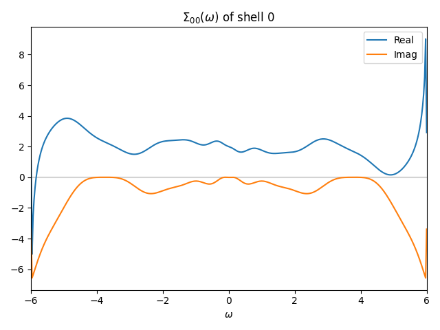
The figure below shows the self-energy in real frequency obtained by analytic continuation (work/post/sigma_w_0_0_0.png).
