Grid search#
In this section, we will explain how to perform a grid-type search and analyze the minimization problem of Himmelblau function.
The grid type search is compatible with MPI. The specific calculation procedure is the same as for minsearch.
The search grid is generated within the program from the input parameters, instead of passing the predefined MeshData.txt to the program.
Location of the sample files#
The sample files are located in sample/analytical/mapper.
The following files are stored in the folder.
input.tomlInput file of the main program.
plot_colormap_2d.pyProgram to visualize the calculation results.
do.shScript prepared for bulk calculation of this tutorial.
Input file#
This section describes the input file for the main program, input.toml. For details, see the “Input file” chapter and Direct parallel search mapper.
[base]
dimension = 2
output_dir = "output"

[solver]
name = "analytical"
function_name = "himmelblau"

[runner]
[runner.log]
interval = 20

[algorithm]
name = "mapper"
seed = 12345

[algorithm.param]
max_list = [6.0, 6.0]
min_list = [-6.0, -6.0]
num_list = [31, 31]
The contents of [base], [solver], and [runner] sections are the same as those for the search by the Nelder-Mead method (minsearch).
[algorithm] section specifies the algorithm to use and its settings.
nameis the name of the algorithm you want to use. In this tutorial we will usemappersince we will be using grid-search method.
In [algorithm.param] section, the parameters for the search grid are specified.
min_listandmax_listare the minimum and the maximum values of each parameter.num_listspecifies the number of grid points along each parameter.
For details on other parameters that are assumed by the default values in this tutorial and can be specified in the input file, please see the Input File chapter.
Calculation execution#
First, move to the folder where the sample files are located. (We assume that you are directly under the directory where you downloaded this software.)
$ cd sample/analytical/mapper
Then, run the main program. The computation time takes only a few seconds on a normal PC.
$ mpiexec -np 4 odatse input.toml | tee log.txt
Here, the calculation is performed using MPI parallelization with 4 processes.
When executed, a folder for each rank will be created under output directory, and the calculation results of each rank will be written.
The standard output will be seen like this.
name            : mapper
seed            : 12345
param.max_list  : [6.0, 6.0]
param.min_list  : [-6.0, -6.0]
param.num_list  : [31, 31]
Iteration : 3/240
Iteration : 3/241
Iteration : 3/240
Iteration : 3/240
Iteration : 6/240
Iteration : 6/241
...
[3] minimum_value: 1.95200000e-01 at 721 (mesh [-2.8, 3.200000000000001])
complete main process : rank 00000003/00000004
end of run
Make ColorMap
The 961 grid points are distributed over 4 processes, so each rank handles 240 or 241 points. The progress is reported every few points, and since the output of the ranks is interleaved, the order of the lines varies from run to run.
Finally, the function values calculated for all the points on the grid will be written to output/ColorMap.txt.
In this case, the following results will be obtained.
-6.000000 -6.000000 890.000000
-5.600000 -6.000000 753.769600
-5.200000 -6.000000 667.241600
-4.800000 -6.000000 622.121600
-4.400000 -6.000000 610.729600
-4.000000 -6.000000 626.000000
-3.600000 -6.000000 661.481600
-3.200000 -6.000000 711.337600
-2.800000 -6.000000 770.345600
...
The first and second columns contain the values of x1 and x2, and the third column contains the function value.
Visualization of calculation results#
By plotting ColorMap.txt, we can estimate the region where the function values are small.
A program plot_colormap_2d.py is prepared to generate such a plot of the two-dimensional space.
$ python3 plot_colormap_2d.py
By executing the above command, output/ColorMapFig.pdf is generated in which the function value evaluated at each grid point is shown as a color map on top of the contour of Himmelblau function.
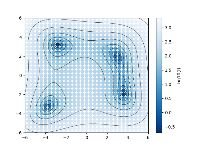
Fig. 3 Color map of the function values in the grid search of the two-dimensional parameter space.#