5.4. Input file for tenes

• File format is TOML format.

• The input file has five sections: parameter, tensor, evolution, observable, correlation.

5.4.1. parameter section

Set various parameters that appear in the calculation, such as the number of updates. This section has five subsections: general, simple_update, full_update, ctm, random.

parameter.general

General parameters for tenes.

Name	Description	Type	Default
mode	Calculation mode	String	\"ground state\"
is_real	Whether to limit all tensors to real valued ones	Boolean	false
iszero_tol	Absolute cutoff value for reading operators	Real	0.0
measure	Whether to calculate and save observables	Boolean	true
measure_interval	Interval of measurement in finite temperature calculation and time evolution process	Integer or list of integers	10
output	Directory for saving result such as physical quantities	String	"output"
tensor_save	Directory for saving optimized tensors	String	""
tensor_load	Directory for loading initial tensors	String	""

• mode

  • Specify the calculation mode

  • "ground state"

    • Search for the ground state of the Hamiltonian

    • tenes_std calculates the imaginary time evolution operator \(U(\tau) = e^{-\tau H}\) from the Hamiltonian \(H\)

  • "time evolution"

    • Calculate the time evolution of the observables from the initial state

    • tenes_std calculates the time evolution operator \(U(t) = e^{-it H}\) from the Hamiltonian \(H\)

  • "finite temperature"

    • Calculate the finite temperature expectation values of the observables

    • tenes_std calculates the imaginary time evolution operator \(U(\tau) = e^{-\tau H}\) from the Hamiltonian \(H\)

• is_real

  • When set to true, the type of elements of the tensor becomes real.

  • If one complex operator is defined at least, calculation will end in errors before starting.

• iszero_tol

  • When the absolute value of operator elements loaded is less than iszero_tol, it is regarded as zero

• meaure

  • When set to false, the stages for measuring and saving observables will be skipped

  • Elapsed time time.dat is always saved

• measure_interval

  • Specify the interval of measurement in time evolution process and finite temperature Calculation

  • Physical quantitites are calculated and saved each after measure_interval updates

• output

  • Save numerical results such as physical quantities to files in this directory

  • Empty means "." (current directory)

• tensor_save

  • Save optimized tensors to files in this directory

  • If empty no tensors will be saved

• tensor_load

  • Read initial tensors from files in this directory

  • If empty no tensors will be loaded

parameter.simple_update

Parameters in the simple update procedure.

Name	Description	Type	Default
tau	(Imaginary) time step \(\tau\) in (imaginary) time evolution operator	Real or list of real	0.01
num_step	Number of simple updates	Integer or list of integers	0
lambda_cutoff	cutoff of the mean field to be considered zero in the simple update	Real	1e-12
gauge_fix	Whether the tensor gauge is fixed	Boolean	false
gauge_maxiter	Maximum number of iterations for fixing gauge	Integer	100
gauge_converge_epsilon	Convergence criteria of iterations for fixing gauge	Real	1e-2

• tau

  • Specify the (imaginary) time step \(\tau\) in (imaginary) time evolution operator

    • tenes_std uses it to calculate the imaginary time evolution operator \(e^{-\tau H}\) from the Hamiltonian

    • tenes uses it to calculate the time of each measurement

      • For finite temperature calculation, note that the inverse temperature increase \(2\tau\) at a step because \(\rho(\beta + 2\tau) = U(\tau)\rho(\beta)\bar{U}(\tau)\)

  • When a list is specified, the time step can be changed for each group of time evolution operators

• num_step

  • Specify the number of simple updates

  • When a list is specified, the number of simple updates can be changed for each group of time evolution operators

parameter.full_update

Parameters in the full update procedure.

Name	Description	Type	Default
tau	(Imaginary) time step \(\tau\) in (imaginary) time evolution operator	Real or list of reals	0.01
num_step	Number of full updates	Integer or list of integers	0
env_cutoff	Cutoff of singular values to be considered as zero when computing environment through full updates	Real	1e-12
inverse_precision	Cutoff of singular values to be considered as zero when computing the pseudoinverse matrix with full update	Real	1e-12
convergence_epsilon	Convergence criteria for truncation optimization with full update	Real	1e-6
iteration_max	Maximum iteration number for truncation optimization on full updates	Integer	100
gauge_fix	Whether the tensor gauge is fixed	Boolean	true
fastfullupdate	Whether the fast full update is adopted	Boolean	true

parameter.ctm

Parameters for corner transfer matrices, CTM.

Name	Description	Type	Default
dimension	Bond Dimension of CTM \(\chi\)	Integer	4
projector_cutoff	Cutoff of singular values to be considered as zero when computing CTM projectors	Real	1e-12
convergence_epsilon	CTM convergence criteria	Real	1e-6
iteration_max	Maximum iteration number of convergence for CTM	Integer	100
projector_corner	Whether to use only the 1/4 corner tensor in the CTM projector calculation	Boolean	true
use_rsvd	Whether to replace SVD with random SVD	Boolean	false
rsvd_oversampling_factor	Ratio of the number of the oversampled elements to that of the obtained elements in random SVD method	Real	2.0
meanfield_env	Use mean field environment obtained through simple update instead of CTM	Boolean	false

For Tensor renomalization group approach using random SVD, please see the following reference, S. Morita, R. Igarashi, H.-H. Zhao, and N. Kawashima, Phys. Rev. E 97, 033310 (2018) .

parameter.random

Parameters for random number generators.

Name	Description	Type	Default
seed	Seed of the pseudo-random number generator used to initialize the tensor	Integer	11

Each MPI process has the own seed as seed plus the process ID (MPI rank).

Example

[parameter]
[parameter.general]
is_real = true
[parameter.simple_update]
num_step = 100
tau = 0.01
[parameter.full_update]
num_step = 0  # No full update
tau = 0.01
[parameter.ctm]
iteration_max = 10
dimension = 9 # CHI

5.4.2. tensor section

Specify the unit cell information (Information of bonds is given in the hamiltonian (tenes_std) and evolution (tenes) sections.). Unit cell has a shape of a rectangular with the size of Lx times Ly. lattice section has an array of subsections unitcell .

Name	Description	Type	Default
L_sub	Unit cell size	Integer or a list of integer	–
skew	Shift value in skew boundary condition	Integer	0

When a list of two integers is passed as L_sub, the first element gives the value of Lx and the second one does Ly. A list of three or more elements causes an error. If L_sub is an integer, both Lx and Ly will have the same value.

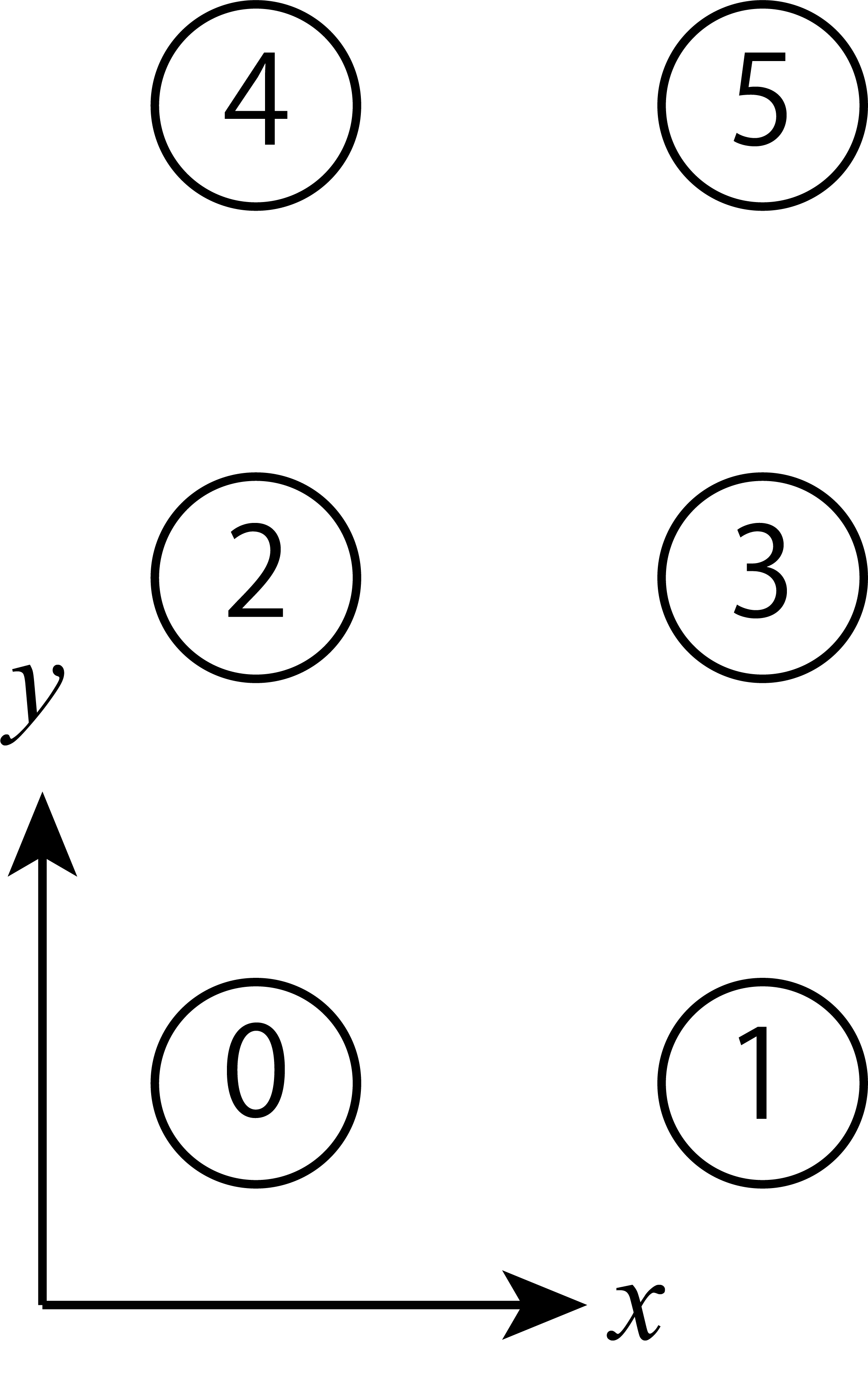
Sites in a unit cell are indexed starting from 0. These are arranged in order from the x direction.

Fig. 5.8 An example for L_sub = [2,3].

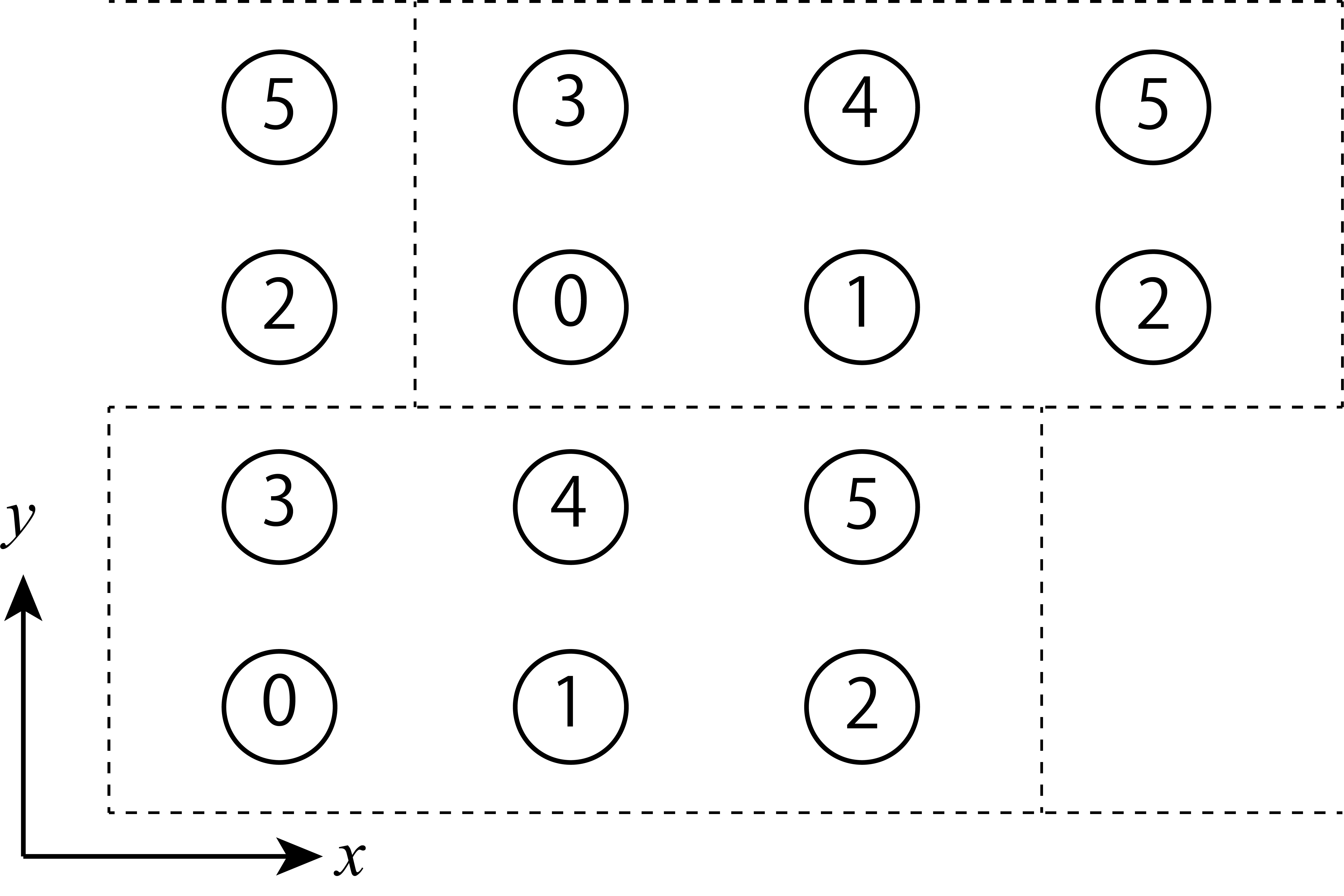
skew is the shift value in the x direction when moving one unit cell in the y direction.

Fig. 5.9 An example for L_sub = [3,2], skew = 1 (ruled line is a separator for unit cell).

tensor.unitcell subsection

The information of site tensors \(T_{ijkl\alpha}^{(n)}\) is specified. Here, \(i, j, k, l\) indicate the index of the virtual bond, \(\alpha\) indicates the index of the physical bond, and \(n\) indicates the site number.

Name	Description	Type
index	Site number	Integer or a list of integer
physical_dim	Dimension of physical bond for a site tensor	Integer
virtual_dim	Dimension of virtual bonds \(D\) for a site tensor	Integer or a list of integer
initial_state	Initial tensor	a list of real
noise	Noise for initial tensor	Real

Multiple sites can be specified at once by setting a list to index. An empty list [] means all sites.

By setting a list to virtual_dim, individual bond dimensions in four directions can be specified. The order is left (-x), top (+y), right (+x), and bottom (-y).

An initial state of a system \(|\Psi\rangle\) is represented as the direct product state of the initial states at each site \(i\), \(|\Psi_i\rangle\):

\[|\Psi\rangle = \otimes_i |\Psi_i\rangle,\]

where \(|\Psi_i\rangle = \sum_\alpha A_\alpha |\alpha\rangle_i\) is the initial state at \(i\) site. Site tensors are initialized to realize this product state with some noise. initial_state specifies (real) values of expansion coefficient \(A_\alpha\), which will be automatically normalized. The tensor itself is initialized such that all elements with a virtual bond index of 0 are \(T_{0000\alpha} = A_\alpha\). The other elements are independently initialized by a uniform random number of [-noise, noise). For example, in the case of \(S=1/2\) , set initial_state = [1.0, 0.0] when you want to set the initial state as the state \(|\Psi_i\rangle = |\uparrow\rangle = |0\rangle\). When you want to set the initial state as the state \(|\Psi_i\rangle = \left(|\uparrow\rangle + |\downarrow\rangle\right)/\sqrt{2}\), set initial_state = [1.0, 1.0].

When an array consisting of only zeros is passed as initil_state, all the elements of the initial tensor will be initialized independently by uniform random value [-noise, noise) .

5.4.3. observable section

Define various settings related to physical quantity measurement. This section has two types of subsections, onesite and twosite.

observable.onesite

Define one-body operators that indicate physical quantities defined at each site \(i\).

Name	Description	type
name	Operator name	String
group	Identification number of operators	Integer
sites	Site number	Integer or a list of integer
dim	Dimension of an operator	Integer
elements	Non-zero elements of an operator	String
coeff	Coefficient of operator (real part)	Float
coeff_im	Coefficient of operator (imaginary part)	Float

name specifies an operator name.

group specifies an identification number of one-site operators.

sites specifies a site number where an operater acts on. By using a list, the operators can be defined on the multiple sites at the same time. An empty list [] means all sites.

dim specifies a dimension of an operator.

elements is a string specifying the non-zero element of an operator. One element is specified by one line consisting of two integers and two floating-point numbers separated by spaces.

• The first two integers are the state numbers before and after the act of the operator, respectively.

• The latter two floats indicate the real and imaginary parts of the elements of the operator, respectively.

coeff and coeff_im are real and imaginary parts of the coefficient of the operator, respectively. If omitted, they are set to 1.0 and 0.0, respectively.

Example

As an example, the case of \(S^z\) operator for S=1/2

\[\begin{split}S^z = \left(\begin{array}{cc} 0.5 & 0.0 \\ 0.0 & -0.5 \end{array}\right)\end{split}\]

is explained.

First, set the name to name = "Sz" and the identification number to group = 0.

Next, if the same operator is used at all sites, set sites = []. Otherwise, for example, if there are sites with different spin length \(S\), specify a specific site number such as sites = [0,1].

The dimension of the operator is dim = 2, because it is the size of the matrix shown above.

Finally, the operator element is defined. When we label two basis on site as \(|\uparrow\rangle = |0\rangle\) and \(|\downarrow\rangle = |1\rangle\), non-zero elements of \(S^z\) are represented as

elements = """
0 0   0.5 0.0
1 1  -0.5 0.0
"""

As a result, \(S^z\) operator for S=1/2 is defined as follows:

[[observable.onesite]]
name = "Sz"
group = 0
sites = []
dim = 2
elements = """
0 0  0.5 0.0
1 1  -0.5 0.0
"""

observable.twosite

Define two-body operators that indicate physical quantities defined on two sites.

Name	Description	Type
name	Operator name	String
group	Identification number of operators	Integer
bonds	Bond	String
dim	Dimension of an operator	Integer
elements	Non-zero elements of an operator	String
ops	Index of onesite operators	A list of integer
coeff	Coefficient of operator (real part)	Float
coeff_im	Coefficient of operator (imaginary part)	Float

name specifies an operator name.

group specifies an identification number of two sites operators.

bonds specifies a string representing the set of site pairs on which the operator acts. One line consisting of three integers means one site pair.

• The first integer is the number of the source site.

• The last two integers are the coordinates (dx, dy) of the other site (target site) from the source site.

  • Both dx and dy must be in the range \(-3 \le dx \le 3\).

dim specifies a dimension of an operator. In other words, the number of possible states of the site where the operator acts on. In the case of interaction between two \(S=1/2\) spins, for example, dim = [2, 2] .

elements is a string specifying the non-zero element of an operator. One element consists of one line consisting of four integers and two floating-point numbers separated by spaces.

• The first two integers are the status numbers of the source site and target site before the operator acts on.

• The next two integers show the status numbers of the source site and target site after the operator acts on.

• The last two floats indicate the real and imaginary parts of the elements of the operator.

Using ops, a two-body operator can be defined as a direct product of the one-body operators defined in observable.onesite. For example, if \(S^z\) is defined as group = 0 in observable.onesite, \(S ^ z_iS ^ z_j\) can be expressed as ops = [0,0].

If both elements and ops are defined, the process will end in error.

coeff and coeff_im are real and imaginary parts of the coefficient of the operator, respectively. If omitted, they are set to 1.0 and 0.0, respectively.

Example

As an example, for the calculation of the energy of the bond Hamiltonian for S=1/2 Heisenberg model on square lattice at Lsub=[2,2] , the way to define two site operators (equal to the Hamiltonian)

\[\mathcal{H}_{ij} = S_i^z S_j^z + \frac{1}{2} \left[S_i^+ S_j^- + S_i^- S_j^+ \right]\]

is explained below.

First, the name and identification number is set as name = "hamiltonian" and group = 0. dim = [2,2] because the state of each site is a superposition of the two states \(|\uparrow\rangle\) and \(|\downarrow\rangle\).

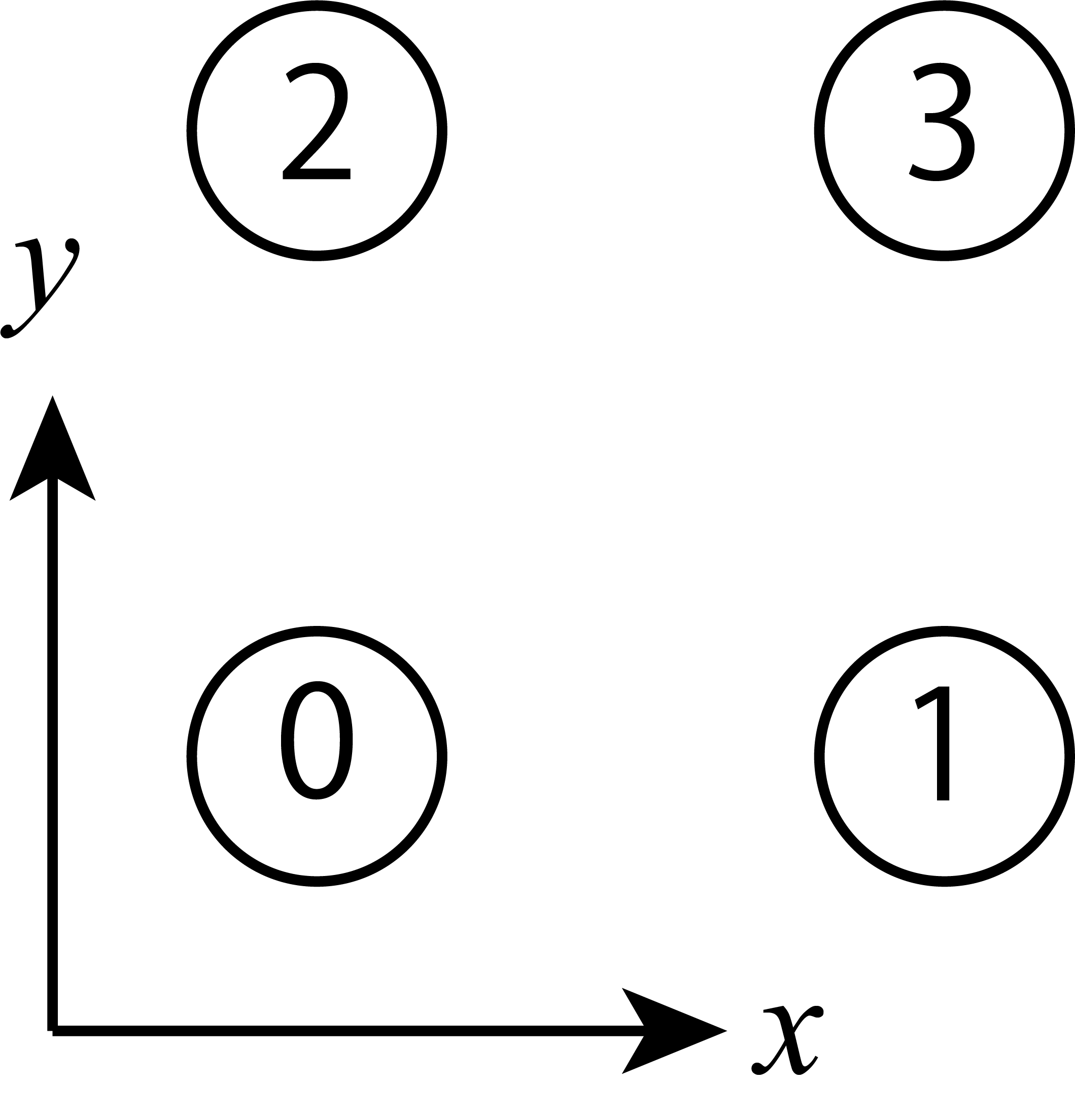
Next, let’s define the bonds. In this case, site indecies are given as shown in bond_22 . The bond connecting 0 and 1 is represented as 0 1 0 because 1 is located at (1,0) from 0. Similarly, The bond connecting 1 and 3 is represented as 1 0 1 because 3 is located at (0,1) from 1.

Fig. 5.10 Site indecies of the S=1/2 Heisenberg model on square lattice at Lsub=[2,2] .

Finally, how to define the elements of the operator is explained. First, the basis of the site is needed to be labeled. Here, we label \(|\uparrow\rangle\) as 0 and \(|\downarrow\rangle\) as 1. Using this basis and label number, for example, one of diagonal elements \(\left\langle \uparrow_i \uparrow_j | \mathcal{H}_{ij} | \uparrow_i \uparrow_j \right\rangle = 1/4\) is specified by 0 0 0 0 0.25 0.0. Likewise, one of off-diagonal elements \(\left\langle \uparrow_i \downarrow_j | \mathcal{H}_{ij} | \downarrow_i \uparrow_j \right\rangle = 1/2\) is specified by 1 0 0 1 0.5 0.0.

As a result, the Heisenberg Hamiltonian for S=1/2 is defined as follows:

[[observable.twosite]]
name = "hamiltonian"
group = 0
dim = [2, 2]
bonds = """
0 0 1
0 1 0
1 0 1
1 1 0
2 0 1
2 1 0
3 0 1
3 1 0
"""
elements = """
0 0 0 0  0.25 0.0
1 0 1 0  -0.25 0.0
0 1 1 0  0.5 0.0
1 0 0 1  0.5 0.0
0 1 0 1  -0.25 0.0
1 1 1 1  0.25 0.0
"""

observable.multisite

Define multi-body operators that indicate physical quantities defined on three or more sites. It is defined as a direct product of one-body operators defined in observable.onesite.

Name	Description	Type
name	Operator name	String
group	Identification number of operators	Integer
multisites	Sites	String
ops	Index of onesite operators	List of integers
coeff	Coefficient of operator (real part)	Float
coeff_im	Coefficient of operator (imaginary part)	Float

name specifies an operator name.

group specifies an identification number of two sites operators.

multisites specifies a string representing the set of sets of sites on which the operator acts. One line consisting of integers means a set sites.

• The first integer is the number of the source site.

• The following integers are the coordinates (dx, dy) of the other sites from the source site.

  • source_site dx2 dy2 dx3 dy3 ... dxN dyN for N-site operator.

  • All sites must be within a square of size \(4 \times 4\).

Using ops, a multi-body operator can be defined as a direct product of the one-body operators defined in observable.onesite. For example, if \(S^z\) is defined as group = 0 in observable.onesite, \(S^z_i S^z_j S^z_k\) can be expressed as ops = [0,0,0].

coeff and coeff_im are real and imaginary parts of the coefficient of the operator, respectively. If omitted, they are set to 1.0 and 0.0, respectively.

5.4.4. evolution section

Specify the imaginary time evolution opetrators used in simple and full updates. One-site and two-sites (nearest neighbor bond) operators can be defined. This section has two subsections: simple and full.

Name	Description	Type
group	Group of the evolution operator	Integer (0-)
site	Index of site	Integer (0-)
source_site	Index of source site	Integer (0-)
source_leg	Direction from source site to target site	Integer (0-3)
dimensions	Dimension of a tensor of imaginary time evolution operator	A list of integers
elements	Non-zero elements of a tensor of imaginary time evolution operator	String

group specifies the group of the evolution operator (the default value is 0). It corresponds to the index of tau and num_steps in parameter.simple_update and parameter.full_update.

site is available for one-site operator, and source_site and source_leg are for two-site operator.

source_leg is specified as an integer from 0 to 3. Defined as 0: -x, 1: + y, 2: + x, 3: -y in the clockwise order from the -x direction.

dimensions is different from dim in observable section, so you need to specify the dimensions of all legs. The order of the legs is source_initial, target_initial, source_final, target_final, just like elements.

Example

[evolution]

# One site
[[evolution.simple]]
site = 0
dimensions = [2, 2]
elements = """
0 0  1.0012507815756226 0.0
1 1  0.9987507809245809 0.0
"""

# Two site
[[evolution.simple]]
source_site = 0
source_leg = 2
dimensions = [2, 2, 2, 2]
elements = """
0 0 0 0  0.9975031223974601 0.0
1 0 1 0  1.0025156589209967 0.0
0 1 1 0  -0.005012536523536871 0.0
1 0 0 1  -0.005012536523536871 0.0
0 1 0 1  1.0025156589209967 0.0
1 1 1 1  0.9975031223974601 0.0
"""

5.4.5. correlation section

In this section, the parameters about the site-site correlation function \(C = \left\langle A(\boldsymbol{r}_0)B(\boldsymbol{r}_0 + \boldsymbol{r}) \right\rangle\) is specified. If you omit this section, no correlation functions will be calculated.

Coordinates \(\boldsymbol{r}, \boldsymbol{r}_0\) measured in the system of square lattice TNS. For example, the coordinate of the right neighbor tensor is \(\boldsymbol{r} = (1,0)\) and that of the top neighbor one is \(\boldsymbol{r} = (0,1)\). TeNeS calculates the correlation functions along the positive direction of \(x\) and \(y\) axis, that is,

\[\boldsymbol{r} = (0,0), (1,0), (2,0), \dots, (r_\text{max}, 0), (0,1), (0,2), \dots, (0, r_\text{max})\]

The coordinate of each site of the unitcell is used as the center coordinate, \(\boldsymbol{r}_0\).

Name	Description	Type
r_max	Maximum distance \(r\) of the correlation function	Integer
operators	Indices of operators A and B to be measured	A list of integer

The operators defined in the observable.onesite section are used.

Example

For example, if \(S^z\) is defined as 0th operator and \(S^x\) is defined as 1st one, then \(S^z(0) S^z(r), S^z(0) S^x(r), S^x(0) S^x(r)\) for \(0 \le r \le 5\) are measured by the following definition:

[correlation]
r_max = 5
operators = [[0,0], [0,1], [1,1]]

5.4.6. correlation_length section

This section describes how to calculate the correlation length \(\xi\).

Name	Description	Type	Default
measure	Whether to calculate \(xi\) or not	Bool	true
num_eigvals	The number of eigenvalues of the transfer matrix to be calculated	Integer	4
maxdim_dense_eigensolver	Maximum dimension of the transfer matrix where the diagonalization method for dense matrices is used	Integer	200
arnoldi_maxdim	Dimension of the Hessenberg matrix generated by the Arnoldi method	Integer	50
arnoldi_restartdim	The number of the initial vectors generated by the restart process of the IRA method	Integer	20
arnoldi_maxiterations	Maximum number of iterations in the IRA method	Integer	1
arnoldi_rtol	Relative tolerance used in the Arnoldi method	Float	1e-10

The correlation length \(\xi\) will be calculated from the dominant eigenvalues of the transfer matrices. If the dimension of the transfer matrix is less than or equal to maxdim_dense_eigensolver, an eigensolver for dense matrices (LAPACK’s *geev routines) will be used. If not, an iterative method, the implicit restart Arnoldi method (IRA method), will be used.

In the IRA method, a Hessenberg matrix with the size of arnoldi_maxdim is generated by the Arnoldi process. Its eigenvalues are approximants of the first arnoldi_maxdim eigenvalues of the original matrix. If not converged, the IRA method restarts the Arnoldi process with the newly generated arnoldi_restartdim initial vectors. In the many cases of the transfer matrices, such a process is not necessary (arnoldi_maxiterations = 1).