5.2. Input file for tenes_simple

• File format is TOML format.

• The input file has four sections : model, parameter, lattice, correlation .

  • The parameter section is copied to the standard mode input.

5.2.1. model section

Specify the model to calculate. In this version, spin system ("spin") and bosonic system ("boson") are defined.

Name	Description	Type	Default
type	Model type (“spin” or “boson”)	String	–

The parameter names such as interactions depend on the model type.

Spin system: "spin"

Hamiltonian is described as

\[\mathcal{H} = \sum_{\langle ij \rangle}\left[\sum_\alpha^{x,y,z} J^\alpha_{ij} S^\alpha_i S^\alpha_j + B \left(\vec{S}_i\cdot\vec{S}_j\right)^2 \right] - \sum_i \sum_\alpha^{x,y,z} h^\alpha S^\alpha_i - \sum_i D \left(S^z_i\right)^2\]

The parameters of the one-body terms are defined as follows.

Name	Description	Type	Default
S	Magnitude of the local spin	Real (integer or half integer)	0.5
hx	Magnetic field along \(S^x\), \(h^x\)	Real	0.0
hy	Magnetic field along \(S^y\), \(h^y\)	Real	0.0
hz	Magnetic field along \(S^z\), \(h^z\)	Real	0.0
D	On-site spin anisotropy \(D\)	Real	0.0

The exchange interaction \(J\) can have a bond dependency.

Name	Description	Type	Default
J0	Exchange interaction of 0th direction nearest neighbor bond	Real	0.0
J1	Exchange interaction of 1st direction nearest neighbor bond	Real	0.0
J2	Exchange interaction of 2nd direction nearest neighbor bond	Real	0.0
J0'	Exchange interaction of 0th direction next nearest neighbor bond	Real	0.0
J1'	Exchange interaction of 1st direction next nearest neighbor bond	Real	0.0
J2'	Exchange interaction of 2nd direction next nearest neighbor bond	Real	0.0
J0''	Exchange interaction of 0th direction third nearest neighbor bond	Real	0.0
J1''	Exchange interaction of 1st direction third nearest neighbor bond	Real	0.0
J2''	Exchange interaction of 2nd direction third nearest neighbor bond	Real	0.0

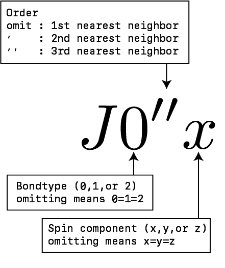
For the next nearest and third nearest neighbor bond, please surround the keyname with the double-quotation marks, ". The bond direction depends on the lattice defined in the lattice section. For a square lattice, for example, coupling constants along two bond directions can be defined, x-direction (0) and y-direction (1). By omitting the direction number, you can specify all directions at once. You can also specify Ising-like interaction by adding one character of xyz at the end. If the same bond or component is specified twice or more, an error will occur.

To summarize,

The biquadratic interaction \(B\) can also have a bond dependency like as \(J\).

Name	Description	Type	Default
B0	Biquadratic interaction of 0th direction nearest neighbor bond	Real	0.0
B1	Biquadratic interaction of 1st direction nearest neighbor bond	Real	0.0
B2	Biquadratic interaction of 2nd direction nearest neighbor bond	Real	0.0
B0'	Biquadratic interaction of 0th direction next nearest neighbor bond	Real	0.0
B1'	Biquadratic interaction of 1st direction next nearest neighbor bond	Real	0.0
B2'	Biquadratic interaction of 2nd direction next nearest neighbor bond	Real	0.0
B0''	Biquadratic interaction of 0th direction third nearest neighbor bond	Real	0.0
B1''	Biquadratic interaction of 1st direction third nearest neighbor bond	Real	0.0
B2''	Biquadratic interaction of 2nd direction third nearest neighbor bond	Real	0.0

One-site operators \(S ^ z\) and \(S ^ x\) are automatically defined. If parameter.general.is_real = false, \(S ^ y\) is also defined. In addition, bond Hamiltonian

\[\mathcal{H}_{ij} = \left[\sum_\alpha^{x,y,z} J^\alpha_{ij} S^\alpha_i S^\alpha_j + B \left(\vec{S}_i\cdot\vec{S}_j\right)^2 \right] - \frac{1}{z} \left[ \sum_\alpha^{x,y,z} h^\alpha \left(S^\alpha_i + S^\alpha_j \right) + D \left(\left(S^z_i\right)^2 + \left(S^z_j\right)^2 \right) \right],\]

and spin correlations on nearest neighbor bonds \(S^\alpha_iS^\alpha_j\) ( \(\alpha=x,y,z\) ) are automatically defined as two-site operators. In the bond Hamiltonian, one body terms (\(h^\alpha\) and \(D\) term) appear only in the nearest neighbor bonds, and \(z\) is the number of the coordinate number.

Bosonic system: "boson"

Hamiltonian is described as

\[\mathcal{H} = \sum_{i<j}\left[ -t_{ij} \left(b^\dagger_i b_j + b^\dagger_j b_i \right) + V_{ij} n_i n_j \right] + \sum_i \left[U\frac{n_i(n_i-1)}{2} - \mu n_i\right],\]

where \(b^\dagger\) and \(b\) are the creation and the annihilation operators of a boson, and \(n = b^\dagger b\) is the number operator.

The parameters of the one-body terms are defined as follows.

Name	Description	Type	Default
nmax	Maximum number of particles on a site	Integer	1
U	Onsite repulsion	Real	0.0
mu	Chemical potential	Real	0.0

The hopping constant \(t\) and the offsite repulsion \(V\) can have a bond dependency.

Name	Description	Type	Default
t0	Hopping of 0th direction nearest neighbor bond	Real	0.0
t1	Hopping of 1st direction nearest neighbor bond	Real	0.0
t2	Hopping of 2nd direction nearest neighbor bond	Real	0.0
t0'	Hopping of 0th direction next nearest neighbor bond	Real	0.0
t1'	Hopping of 1st direction next nearest neighbor bond	Real	0.0
t2'	Hopping of 2nd direction next nearest neighbor bond	Real	0.0
t0''	Hopping of 0th direction third nearest neighbor bond	Real	0.0
t1''	Hopping of 1st direction third nearest neighbor bond	Real	0.0
t2''	Hopping of 2nd direction third nearest neighbor bond	Real	0.0
V0	Offsite repulsion of 0th direction nearest neighbor bond	Real	0.0
V1	Offsite repulsion of 1st direction nearest neighbor bond	Real	0.0
V2	Offsite repulsion of 2nd direction nearest neighbor bond	Real	0.0
V0'	Offsite repulsion of 0th direction next nearest neighbor bond	Real	0.0
V1'	Offsite repulsion of 1st direction next nearest neighbor bond	Real	0.0
V2'	Offsite repulsion of 2nd direction next nearest neighbor bond	Real	0.0
V0''	Offsite repulsion of 0th direction third nearest neighbor bond	Real	0.0
V1''	Offsite repulsion of 1st direction third nearest neighbor bond	Real	0.0
V2''	Offsite repulsion of 2nd direction third nearest neighbor bond	Real	0.0

The bond direction depends on the lattice defined in the lattice section. For a square lattice, for example, coupling constants along two bond directions can be defined, x-direction (0) and y-direction (1). By omitting the direction number, you can specify all directions at once.

One-site operators \(n\), \(b\), and \(b^\dagger\) are automatically defined. In addition, bond Hamiltonian

\[\mathcal{H}_{ij} = \left[ -t_{ij} \left(b^\dagger_i b_j + b^\dagger_j b_i \right) + V_{ij} n_i n_j \right] + \frac{1}{z} \left[\left(U\frac{n_i(n_i-1)}{2} - \mu n_i\right) + (i \leftrightarrow j)\right]\]

and short range correlations on nearest neighbor bonds \(n_i n_j\), \(b^\dagger_i b_j\), and \(b_i b^\dagger_j\) are automatically defined as two-site operators. In the bond Hamiltonian, one body terms (\(U\) and \(\mu\) term) appear only in the nearest neighbor bonds, and \(z\) is the number of the coordinate number.

5.2.2. lattice section

Specify the lattices to calculate. Square, triangular, honeycomb, and Kagome lattices are defined.

Name	Description	Type	Default
type	lattice name (square, triangular or honeycomb lattice)	String	–
L	Unit cell size in x direction	Integer	–
W	Unit cell size in y direction	Integer	L
virtual_dim	Bond dimension	Integer	–
initial	Inital state	String	random
noise	Noise for elements in initial tensor	Real	1e-2

initial and noise are parameters that determine the initial state of the wave function. If tensor_load is set in parameter.general, initial is ignored.

• initial

  • "ferro" : Ferromagnetic state

    • In spin system, all sites has \(S^z = S\)

    • In bosonic system, all sites has \(n = n_{\text{max}}\) particles

  • "antiferro" : Antiferromagnetic state

    • In spin system, for square lattice and honeycomb lattice, the Neel order state (\(S^z = S\) for the A sublattice and \(S^z = -S\) for the B sublattice), and for triangular lattice and kagome lattice, the 120 degree order state (spins on sites belonging to the A, B, and C sublattice are pointing to \((\theta, \phi) = (0,0), (2\pi/3, 0)\) and \((2\pi/3, \pi)\) direction, respectively.)

    • In bosonic system, sites belonging to one sublattice have \(n_\text{max}\) particles and the other sites have no particles.

  • "random" : Random state

• noise

  • The amount of fluctuation in the elements of the initial tensor

Square lattice

A square lattice type = "square lattice" consists of L sites in the \((1,0)\) direction and W sites in the \((0,1)\) direction. As a concrete example, Fig. 5.1 (a) shows the structure for L=3, W=3. In addition, the definitions of the first, second and third nearest neighbor bonds are shown in Fig. 5.1 (b), (c), and (d), respectively. The blue line represents a bond of bondtype = 0 and the red line represents a bond of bondtype = 1.

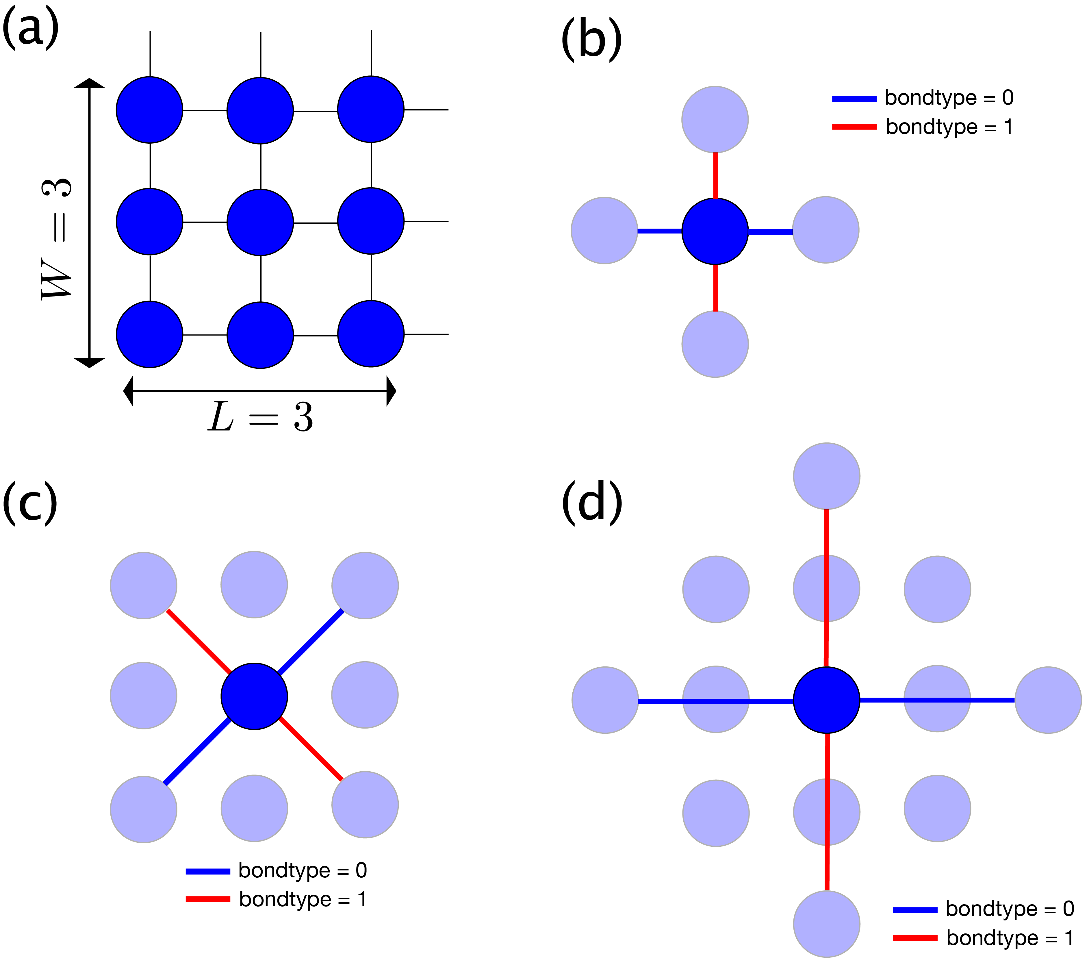
Fig. 5.1 Square lattice. (a) Site structure with L=3, W=3 (b) Nearest neighbor bonds. bondtype=0 (blue) bond extends in the 0 degree direction and bondtype=1 (red) one in the 90 degree direction. (c) Second nearest neighbor bonds. bondtype=0 (blue) bond extends in the 45 degree direction and bondtype=1 (red) one in the -45 degree direction. (d) Third nearest neighbor bonds. bondtype=0 (blue) bond extends in the 0 degree direction and bondtype=1 (red) one in the 90 degree direction.

Triangular lattice

A triangular lattice type = "triangular lattice" consists of L sites in the \((1,0)\) direction and W sites in the \((1/2, \sqrt{3}/2)\) direction. As a concrete example, Fig. 5.2 (a) shows the structure for L=3, W=3. In addition, the definitions of the first, second and third nearest neighbor bonds are shown in Fig. 5.2 (b), (c), and (d), respectively. The blue, red, and green lines represent bonds of bondtype = 0, 1, and 2, respectively. (e) shows the corresponding square TPS with L=3, W=3.

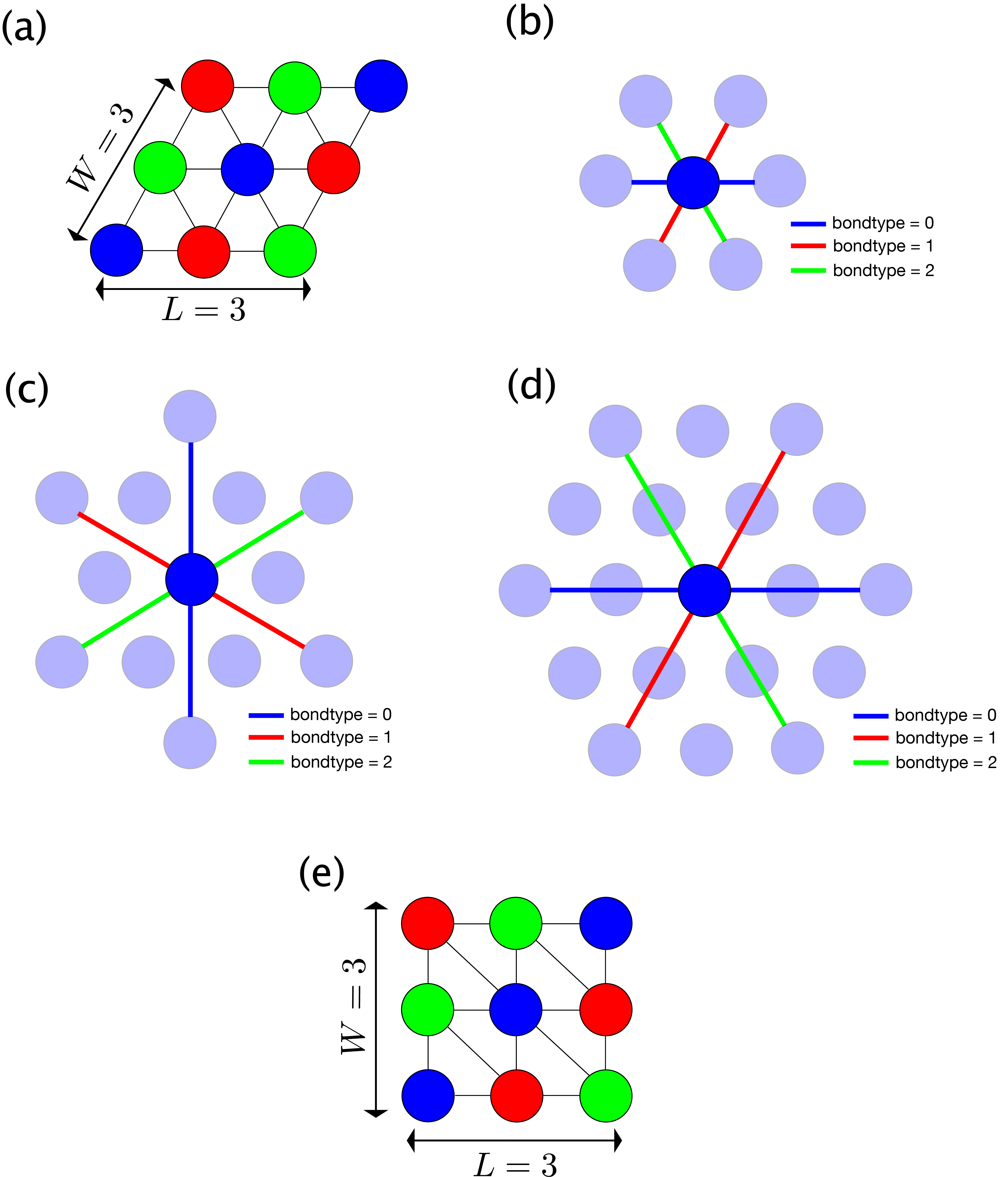
Fig. 5.2 Triangular lattice. (a) Site structure with L=3, W=3 (b) Nearest neighbor bonds. bondtype=0 (blue) bond extends in the 0 degree direction, bondtype=1 (red) one in the 60 degree direction, and bondtype=2 (green) one in the 120 degree direction. (c) Second nearest neighbor bonds. bondtype=0 (blue) bond extends in the 90 degree direction, bondtype=1 (red) one in the -30 degree direction, and bondtype=2 (green) one in the 30 degree direction. (d) Third nearest neighbor bonds. bondtype=0 (blue) bond extends in the 0 degree direction, bondtype=1 (red) one in the 60 degree direction, and bondtype=2 (green) one in the 120 degree direction. (e) Corrensponding square TPS of the triangular lattice with L=3, W=3.

Honeycomb lattice

In a honeycomb lattice type = "honeycomb lattice", units consisting of two sites of coordinates \((0, 0)\) and \((\sqrt{3}/2, 1/2)\) are arranged with L units in the \((\sqrt{3},0)\) direction and W units in the \((1/2, 3/2)\) direction. As a concrete example, Fig. 5.3 (a) shows the structure for L=2, W=2. In addition, the definitions of the first, second and third nearest neighbor bonds are shown in Fig. 5.3 (b), (c), and (d), respectively. The blue, red, and green lines represent bonds of bondtype = 0, 1, and 2, respectively. (e) shows the corresponding square TPS with L=2, W=2.

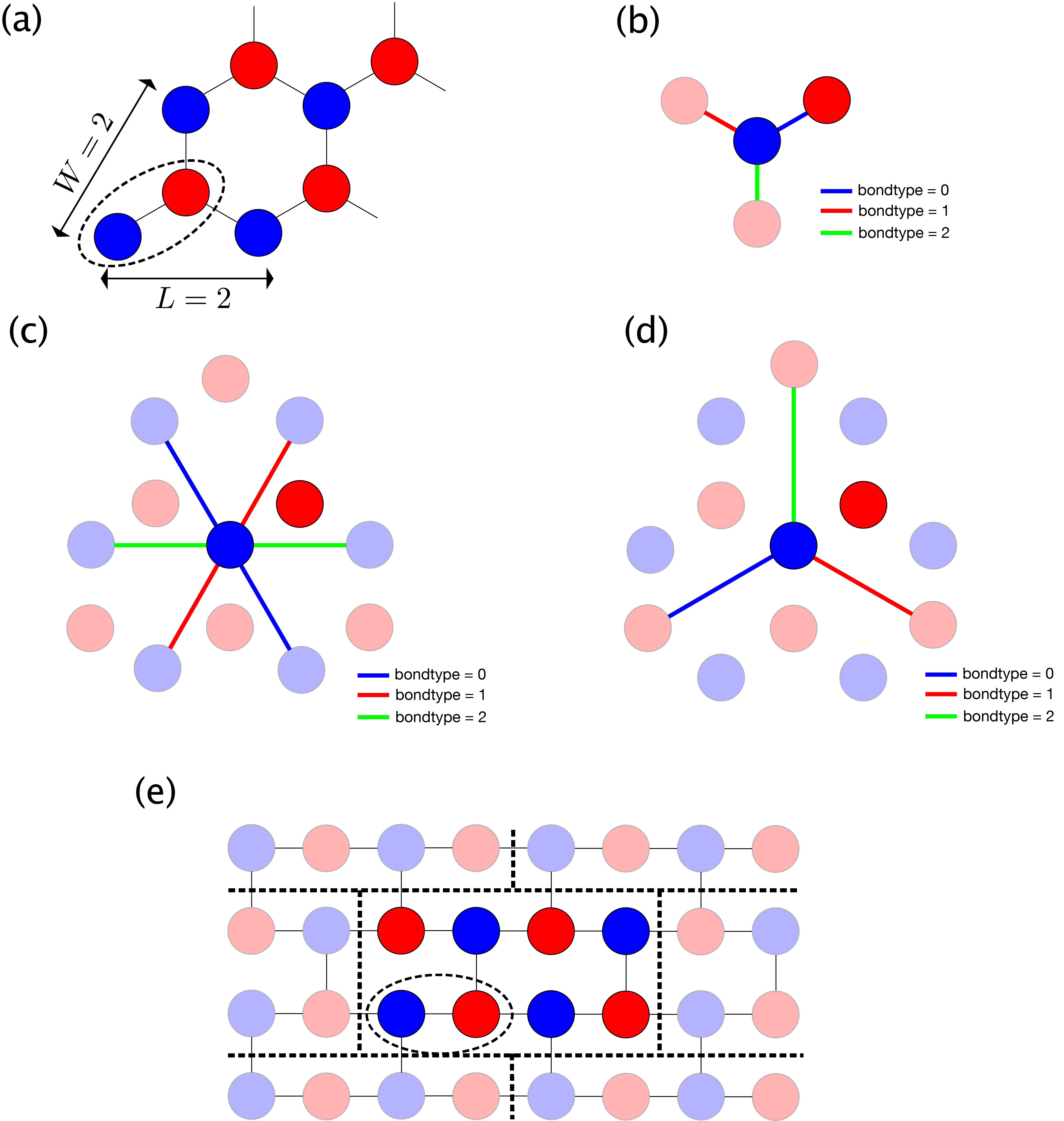
Fig. 5.3 Honeycomb lattice. (a) Site structure with L=2, W=2. The dashed ellipse denotes one unit. (b) Nearest neighbor bonds. bondtype=0 (blue) bond extends in the 30 degree direction, bondtype=1 (red) one in the 150 degree direction, and bondtype=2 (green) one in the -90 degree direction. (c) Second nearest neighbor bonds. bondtype=0 (blue) bond extends in the 120 degree direction, bondtype=1 (red) one in the 60 degree direction, and bondtype=2 (green) one in the 0 degree direction. (d) Third nearest neighbor bonds. bondtype=0 (blue) bond extends in the -30 degree direction, bondtype=1 (red) one in the -150 degree direction, and bondtype=2 (green) one in the 90 degree direction. (e) Corresponding square TPS of the honeycomb lattice with L=2, W=2. Note that the most top-right red tensor in the honeycomb lattice moves to the most top-left position, and the boundary condition is skewed.

Kagome lattice

In a kagome lattice type = "kagome lattice", units consisting of three sites of coordinates \((0, 0)\), \((1, 0)\), and \((1/2, \sqrt{3}/2)\) are arranged with L units in the \((2,0)\) direction and W units in the \((1,\sqrt{3})\) direction. As a concrete example, Fig. 5.4 (a) shows the structure for L=2, W=2. In addition, the definitions of the first, second and third nearest neighbor bonds are shown in Fig. 5.4 (b), (c), and (d), respectively. The blue and the red lines represent bonds of bondtype = 0, and 1, respectively. (e) shows the corresponding square TPS with L=2, W=2.

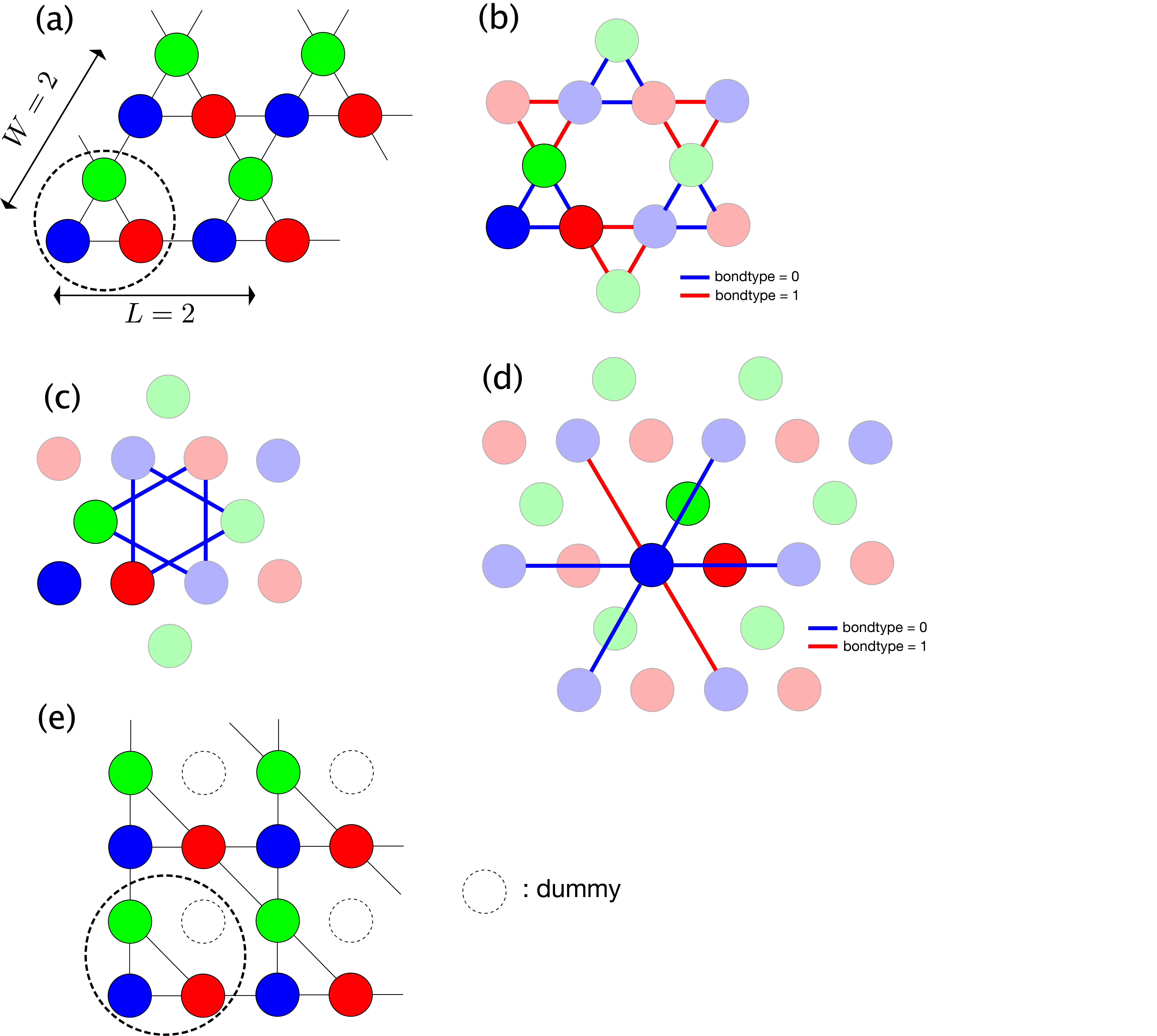
Fig. 5.4 Kagome lattice. (a) Site structure with L=2, W=2. The dashed circle denotes one unit. (b) Nearest neighbor bonds. bondtype=0 (blue) bonds form upper triangle and bondtype=1 (red) bonds form lowertriangle. (c) Second nearest neighbor bonds. (d) Third nearest neighbor bonds. bondtype=0 (blue) bond passes over a site and bondtype=1 (red) one does not. (e) Corresponding square TPS of the kagome lattice with L=2, W=2. The white circles are the dummy tensors with bonds of dimension one.

5.2.3. parameter section

Parameters defined in this section is not used in tenes_simple but they are copied to the input file of tenes_std.

Set various parameters that appear in the calculation, such as the number of updates. This section has five subsections: general, simple_update, full_update, ctm, random.

parameter.general

General parameters for tenes.

Name	Description	Type	Default
mode	Calculation mode	String	\"ground state\"
is_real	Whether to limit all tensors to real valued ones	Boolean	false
iszero_tol	Absolute cutoff value for reading operators	Real	0.0
measure	Whether to calculate and save observables	Boolean	true
measure_interval	Interval of measurement in finite temperature calculation and time evolution process	Integer or list of integers	10
output	Directory for saving result such as physical quantities	String	"output"
tensor_save	Directory for saving optimized tensors	String	""
tensor_load	Directory for loading initial tensors	String	""

• mode

  • Specify the calculation mode

  • "ground state"

    • Search for the ground state of the Hamiltonian

    • tenes_std calculates the imaginary time evolution operator \(U(\tau) = e^{-\tau H}\) from the Hamiltonian \(H\)

  • "time evolution"

    • Calculate the time evolution of the observables from the initial state

    • tenes_std calculates the time evolution operator \(U(t) = e^{-it H}\) from the Hamiltonian \(H\)

  • "finite temperature"

    • Calculate the finite temperature expectation values of the observables

    • tenes_std calculates the imaginary time evolution operator \(U(\tau) = e^{-\tau H}\) from the Hamiltonian \(H\)

• is_real

  • When set to true, the type of elements of the tensor becomes real.

  • If one complex operator is defined at least, calculation will end in errors before starting.

• iszero_tol

  • When the absolute value of operator elements loaded is less than iszero_tol, it is regarded as zero

• meaure

  • When set to false, the stages for measuring and saving observables will be skipped

  • Elapsed time time.dat is always saved

• measure_interval

  • Specify the interval of measurement in time evolution process and finite temperature Calculation

  • Physical quantitites are calculated and saved each after measure_interval updates

• output

  • Save numerical results such as physical quantities to files in this directory

  • Empty means "." (current directory)

• tensor_save

  • Save optimized tensors to files in this directory

  • If empty no tensors will be saved

• tensor_load

  • Read initial tensors from files in this directory

  • If empty no tensors will be loaded

parameter.simple_update

Parameters in the simple update procedure.

Name	Description	Type	Default
tau	(Imaginary) time step \(\tau\) in (imaginary) time evolution operator	Real or list of real	0.01
num_step	Number of simple updates	Integer or list of integers	0
lambda_cutoff	cutoff of the mean field to be considered zero in the simple update	Real	1e-12
gauge_fix	Whether the tensor gauge is fixed	Boolean	false
gauge_maxiter	Maximum number of iterations for fixing gauge	Integer	100
gauge_converge_epsilon	Convergence criteria of iterations for fixing gauge	Real	1e-2

• tau

  • Specify the (imaginary) time step \(\tau\) in (imaginary) time evolution operator

    • tenes_std uses it to calculate the imaginary time evolution operator \(e^{-\tau H}\) from the Hamiltonian

    • tenes uses it to calculate the time of each measurement

      • For finite temperature calculation, note that the inverse temperature increase \(2\tau\) at a step because \(\rho(\beta + 2\tau) = U(\tau)\rho(\beta)\bar{U}(\tau)\)

  • When a list is specified, the time step can be changed for each group of time evolution operators

• num_step

  • Specify the number of simple updates

  • When a list is specified, the number of simple updates can be changed for each group of time evolution operators

parameter.full_update

Parameters in the full update procedure.

Name	Description	Type	Default
tau	(Imaginary) time step \(\tau\) in (imaginary) time evolution operator	Real or list of reals	0.01
num_step	Number of full updates	Integer or list of integers	0
env_cutoff	Cutoff of singular values to be considered as zero when computing environment through full updates	Real	1e-12
inverse_precision	Cutoff of singular values to be considered as zero when computing the pseudoinverse matrix with full update	Real	1e-12
convergence_epsilon	Convergence criteria for truncation optimization with full update	Real	1e-6
iteration_max	Maximum iteration number for truncation optimization on full updates	Integer	100
gauge_fix	Whether the tensor gauge is fixed	Boolean	true
fastfullupdate	Whether the fast full update is adopted	Boolean	true

parameter.ctm

Parameters for corner transfer matrices, CTM.

Name	Description	Type	Default
dimension	Bond Dimension of CTM \(\chi\)	Integer	4
projector_cutoff	Cutoff of singular values to be considered as zero when computing CTM projectors	Real	1e-12
convergence_epsilon	CTM convergence criteria	Real	1e-6
iteration_max	Maximum iteration number of convergence for CTM	Integer	100
projector_corner	Whether to use only the 1/4 corner tensor in the CTM projector calculation	Boolean	true
use_rsvd	Whether to replace SVD with random SVD	Boolean	false
rsvd_oversampling_factor	Ratio of the number of the oversampled elements to that of the obtained elements in random SVD method	Real	2.0
meanfield_env	Use mean field environment obtained through simple update instead of CTM	Boolean	false

For Tensor renomalization group approach using random SVD, please see the following reference, S. Morita, R. Igarashi, H.-H. Zhao, and N. Kawashima, Phys. Rev. E 97, 033310 (2018) .

parameter.random

Parameters for random number generators.

Name	Description	Type	Default
seed	Seed of the pseudo-random number generator used to initialize the tensor	Integer	11

Each MPI process has the own seed as seed plus the process ID (MPI rank).

Example

[parameter]
[parameter.general]
is_real = true
[parameter.simple_update]
num_step = 100
tau = 0.01
[parameter.full_update]
num_step = 0  # No full update
tau = 0.01
[parameter.ctm]
iteration_max = 10
dimension = 9 # CHI

5.2.4. correlation section

For tenes_simple , correlation functions \(C = \langle A(0)B(r)\rangle\) are not calculated by default. For calculating correlation functions, they have to be specified in the same file format as the input file of tenes. For details, See correlation section Input file for tenes.

5.2.5. correlation_length section

Parameters defined in this section is not used in tenes_simple but they are copied to the input file of tenes_std.

This section describes how to calculate the correlation length \(\xi\).

Name	Description	Type	Default
measure	Whether to calculate \(xi\) or not	Bool	true
num_eigvals	The number of eigenvalues of the transfer matrix to be calculated	Integer	4
maxdim_dense_eigensolver	Maximum dimension of the transfer matrix where the diagonalization method for dense matrices is used	Integer	200
arnoldi_maxdim	Dimension of the Hessenberg matrix generated by the Arnoldi method	Integer	50
arnoldi_restartdim	The number of the initial vectors generated by the restart process of the IRA method	Integer	20
arnoldi_maxiterations	Maximum number of iterations in the IRA method	Integer	1
arnoldi_rtol	Relative tolerance used in the Arnoldi method	Float	1e-10

The correlation length \(\xi\) will be calculated from the dominant eigenvalues of the transfer matrices. If the dimension of the transfer matrix is less than or equal to maxdim_dense_eigensolver, an eigensolver for dense matrices (LAPACK’s *geev routines) will be used. If not, an iterative method, the implicit restart Arnoldi method (IRA method), will be used.

In the IRA method, a Hessenberg matrix with the size of arnoldi_maxdim is generated by the Arnoldi process. Its eigenvalues are approximants of the first arnoldi_maxdim eigenvalues of the original matrix. If not converged, the IRA method restarts the Arnoldi process with the newly generated arnoldi_restartdim initial vectors. In the many cases of the transfer matrices, such a process is not necessary (arnoldi_maxiterations = 1).