8. Algorithm
abICS is designed for combining parallel extended ensemble methods with arbitrary energy calculators. At present, the replica exchange Monte Carlo method and the population annealing Monte Carlo method are implemented.
Overview of abICS
8.1. Replica exchange Monte Carlo method
A disadvantage of the widely-used Metropolis Monte Carlo algorithm is that it tends to get stuck in local minima. The replica exchange approach aims to overcome this problem by considering multiple copies, or replicas, of the system under study. The algorithm may be described roughly as follows (see references below for more accurate descriptions). Monte Carlo sampling is performed on each replica independently at varying temperatures. At preset intervals, the temperatures are exchanged according to a Metropolis criterion that essentially assigns lower temperatures to replicas that happen to have lower energies. This allows an efficient sampling of the global configuration space using replicas at higher temperatures and accurate sampling of the local energy landscape at lower temperatures.
In abICS, parameters related to the replica exchange Monte Carlo method are specified in the [replica] section of the input file.
By setting the lower limit of the replica temperature to \(T_s =\) kTstart , the upper limit to \(T_e =\) kTend, and the number of replicas to \(N_r =\) nreplicas,
\(N_r\) replica systems with different temperatures ( \(T_0, T_1, \cdots T_{N_r-1}\)) are sampled, where
In abICS, using nprocs_per_replica, the number of parallel solver processes that performs the calculation on each replica can be specified.
The number of Monte Carlo steps is specified by nsteps, and the exchange transition probability \(R\) for each RXtrial_frequency step is defined as
where \(X_i\) is the state for \(i\) -th replica system. In abICS, the exchange transition is tried between replicas with adjacent temperatures.
The temperature exchange \(T_i \leftrightarrow T_{k}\) is performed with the exchange transition probability \(R\).
Physical quantities such as the total energy is measured at each sample_frequency step.
About replica exchange Monte Carlo method
8.2. Population Annealing Monte Carlo
The simulated annealing (SA) method is one of the Monte Carlo method for searching for the ground state. SA performs an ordinally MC sampling under a fixed temperature, and decreases temperature after a given number of MC steps finished. SA first searches a whole space, and then searches narrower regions gradually as temperature decreases. A disadvabtage of SA is that a change of temperature distorts the distribution from equilibrium, and hence thermalization steps are necessary to obtain canonical average of observables for each temperature. The annealed importance sampling (AIS) method overcomes this problem. AIS performs SA on many replicas in parallel, and compensates for deviation of distributions by introducing an extra weight. This weight (Neal-Jarzynski weight) is appropriately defined so that the weighted average of observables over replicas is just the canonical average for each temperature. In AIS, the variance of the NJ weights increases as the simulation progresses, and then only some replicas contribute to the average, in other words, an effective number of replicas decreases. Therefore, the population annealing Monte Carlo (PAMC) method resamples the replicas periodically so that the distribution of replicas is propotional to the NJ weights and resets the weights to 1.
8.3. About configuration and update
Here, the outline of the definition of the configuration in abICS and the update by the Monte Carlo method are explained using Fig. 8.1 as an example.
(a)-(c) are schematic figures of unitcell, base_structure, and defect_structure, where blue, green, and black circles are the atomic types defined by base_structure, respectively. The star symbol indicates the location of the defects defined by defect_structure.
(d) is a schematic figure for specifying the atomic species in base_structure. Here, three atomic species of blue, green, and black are defined. How each atom is arranged is defined by coords for each atom type.
(e) is a schematic figure for specifying the group of atoms to be located at the defect position with defect_structure. orange defines a group consisting of four atoms composed of two types of atoms, and purple forms a group of three atoms composed of three types of atoms. These groups are placed at defect points specified by defect_structure.coords. The arrangement of atoms in each group can be specified by coords in the defect_structure.groups section.
defect_structure can be defined multiple times. Groups of each defect_structure will be placed at points of each one.
(f) is a schematic figure about the update of the Monte Carlo method. In the update, there are two patterns, one that swaps two atom groups of different type
, and the other that changes the orientation within the atom group without changing the arrangement. The type of updates is automatically selected with 1/2 probability. The energy is calculated with the specified solver from the proposed configuration \(X_ {trial}\) and then the adoption rate \(P (X_i \rightarrow X_ {trial})\) is calculated.
When the grand canonical sampling is turned on by the parameter sampling.enable_grandcanonical, the additional update patterns are also introduced in which the atom groups are added from or removed to the reservoir. The numbers of the atom groups are controlled by the chemical potentials config.chemical_potential for each atom group or a set of groups simultaneously.
The configuration is updated by the Metropolis-Hastings algorithm according to the adoption rate calculated from the differences of the energy and the particle numbers between the original and proposed configurations as
where \(\Delta W = Q(X_\text{trial}\to X_i)/Q(X_i\to X_\text{trial})\) denotes the weight factor derived from the proposal distribution \(Q(X\to X^\prime)\) from a configuration \(X\) to \(X^\prime\).
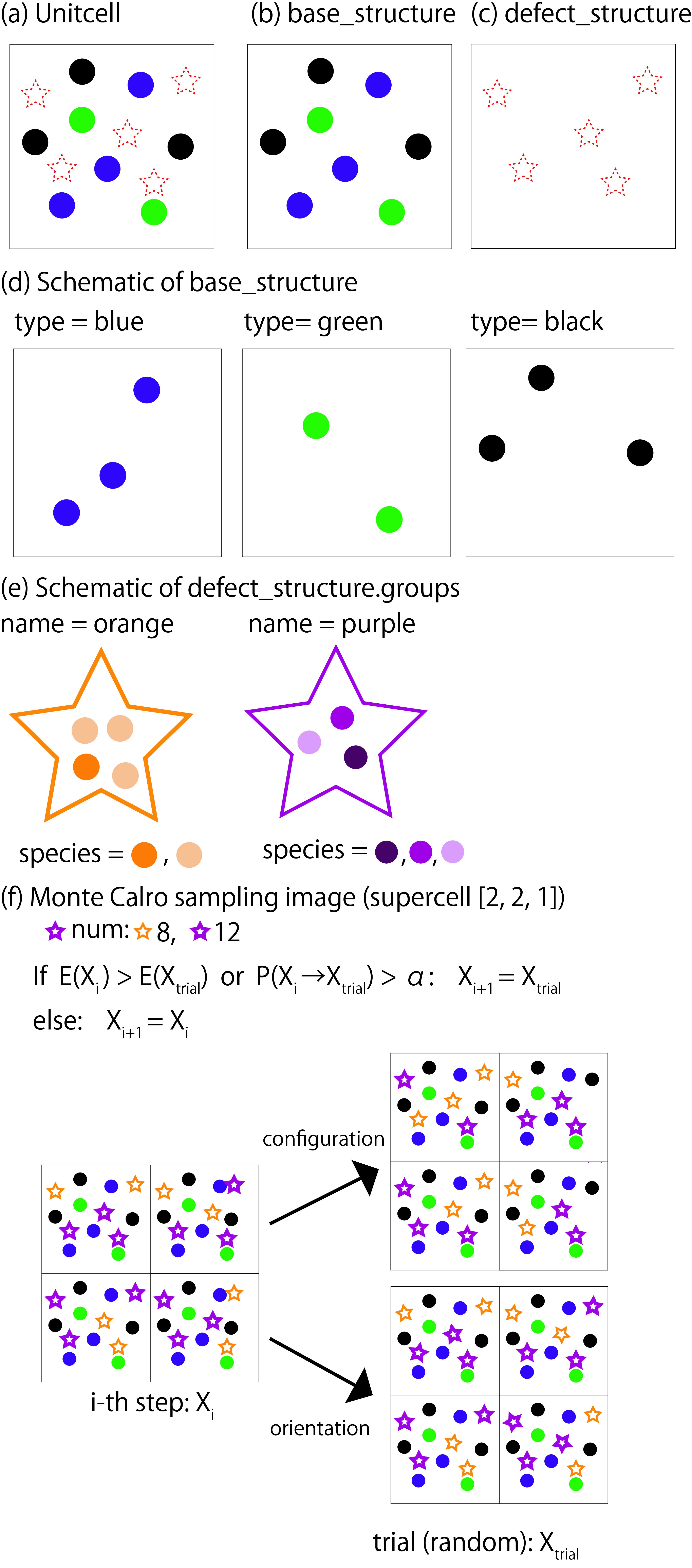
Fig. 8.1 (a)-(e) Definition of lattice in abICS. (f) A schematic of MonteCarlo method. Details are described in the text.