3. Basic Usage
3.1. Active learning
abICS was originally developed for directly combining first-principles calculations with replica-exchange Monte Carlo methods to perform configurational sampling, but the scale of the models and the number of steps that can be calculated are limited by the large computational cost of first-principles calculations. In contrast, Ver. 2 implements an active learning method to construct a neural network model that can rapidly predict the energy after structural optimization, dramatically improving the sampling speed [Kasamatsu et al., 2022] .
The general flow of the active learning method implemented in abICS is as follows.
Perform ab initio calculations on a large number of randomly generated atomic configurations and prepare training data (correspondence between configurations and energies).
Build a neural network model that predicts energy from atomic configurations using the prepared training data.
Perform statistical thermodynamic sampling of atomic configurations using a replica exchange Monte Carlo method with a neural network model.
Evaluate the accuracy of the neural network model by sampling the ion configurations that appear in the Monte Carlo calculations and performing ab initio calculations on each of them.
If the accuracy is not sufficient, add the results calculated in 4. to the training data and repeat from 2.
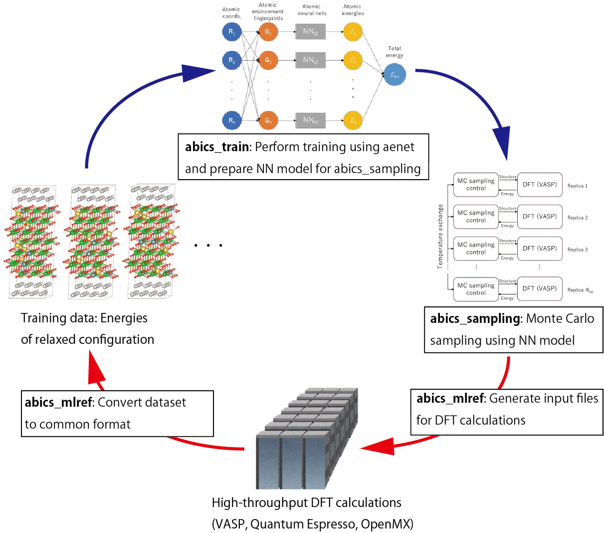
Schematic of the active learning procedure using abICS
3.2. Preparing an abICS control file
First, we have to prepare an input file that controls the entire abICS framework. The input file of abICS is comprised of the following five sections:
[sampling] section specifies the parameters of the replica exchange Monte Carlo part, such as the number of replicas, the temperature range, and the number of Monte Carlo steps. In addition, [sampling.solver] subsection specifies the parameters for the (first principle calculation) solver, including the type of solver (VASP, QE,…), the path to the solver, and the directory containing immutable input files.
[mlref] section specifies options for extracting only atomic configurations from the sampling results in order to evaluate the accuracy of the neural network model and to expand the training data. In addition, for generating training data, [mlref.solver] subsection specifies the parameters for the (first principle calculation) solver, including the type of solver (VASP, QE,…), the path to the solver, and the directory containing immutable input files. This section is used for
abics_mlref.[train] section specifies optinons for making a trainer to learn a placement energy prediction model from training data. This section is used for
abics_train.[observer] section specifies the type of physical quantity to be calculated.
[config] section specifies the configuration of the alloy, etc.
For details, see Input Files Format . The following is an example of an input file selecting aenet as a solver.
3.3. Preparing a reference file for first-principles solvers
The user must prepare reference input file(s) for first-principles solvers that are used for
generating the training data according to the input format of the solver.
The path of the reference file is specified by base_input_dir in the [mlref.solver] section in the abICS input file (see below).
The coordinate information should not be written here; it will be written by abICS.
The following is an example of a QE reference file.
&CONTROL
  calculation = 'relax'
  tstress = .false.
  tprnfor = .false.
  pseudo_dir = './pseudo'
  disk_io = 'low'
  wf_collect = .false.
/
&SYSTEM
  ecutwfc      =  60.0
  occupations  = "smearing"
  smearing     = "gauss"
  degauss      = 0.01
/
&electrons
  mixing_beta = 0.7
  conv_thr = 1.0d-8
  electron_maxstep = 100
/
&ions
/
ATOMIC_SPECIES
Al 26.981 Al.pbe-nl-kjpaw_psl.1.0.0.UPF
Mg 24.305 Mg.pbe-spnl-kjpaw_psl.1.0.0.UPF
O  16.000 O.pbe-n-kjpaw_psl.1.0.0.UPF
ATOMIC_POSITIONS crystal

K_POINTS gamma
3.3.1. Specific notes for first-principles solvers
Every setting other than those pertaining to the atomic coordinates should be set in the solver reference input file. However, the specification of atoms to be relaxed can be controlled by abICS. To enable the structural optimization option, please set the option to do structural optimization in the reference file of the solver, and also specify the related parameters such as the total number of steps for relaxation. Furthermore, to interoperate with abICS, there are a few rules regarding the file name and contents of the reference file for each solver. We’ll explain them below.
VASP
URL : https://www.vasp.at
Reference file rules
Please prepare INCAR, POTCAR, KPOINTS files.
In POTCAR file, please arrange the atoms in alphabetical order.
The POSCAR file is basically not needed, but maybe needed depending on the version of
pymatgen. In that case, please prepare a suitable file.
Quantum Espresso
Available version: 6.2 or higher
“Old XML” format is not available
Reference file rules
Please set the reference file name as
scf.in.calculationoption must bescforrelax.If the calculation is done only at \(\Gamma\) point, the calculation becomes fast if you set
Gammainkpoints.
OpenMX
Available version: 3.9
Reference file rule
Please set the reference file name as
base.dat.
3.4. Preparing a reference file for training and evaluating the machine learning model
The user must prepare a reference file according to the input format of the
machine learning model trainer and calculator to be used (only aenet is supported at the moment).
The path of the reference file is specified by base_input_dir in the [solver] section in the abICS input file (see below).
The coordinate information should not be written here because it will obviously change in the course of the simulation.
The lattice sites are specified in a separate abICS input file (see below),
and abICS will take care of generating the coordinates section at each sampling step.
3.4.1. Machine learning trainer/calculator-specific notes
abICS control file
In the
[solver]section, setperturbbe 0.0.
type = "aenet"
perturb = 0.0
aenet
URL : http://ann.atomistic.net
Checked with aenet 2.0.4.
Reference file rules
Place the input files for aenet in the
generate,train, andpredictdirectories in the directory which is set in thebase_input_dirof the[trainer]section.aenet compiles the atomic configuration and energy data for training into an intermediate binary format that is converted to atomic environment descriptor-energy relationships before training. Please place the input files for this conversion
generate.xin thegeneratedirectory.Place an input file for
train.xin thetraindirectory that reads the training data generated bygenerate.xand trains. The file should be namedtrain.in.Place the input file
predict.inforpredict.xin thepredictdirectory to evaluate the energy for the input coordinates using the trained potential model.
NequIP
Checked with nequip 0.6.1.
Reference file(For specific examples of reference files, see the tutorial)
Place the input file for NequIP
input.yamlin thetraindirectory in the directory set in thebase_input_dirof the[trainer]section.Set the RATIO of training data and validation data in
n_trainandn_val. For example, if you setn_train = 80%andn_val = 20%, the ratio of training data and validation data will be 80% and 20%, respectively.
MLIP-3
Checked with commit hash 5f6970e3966c5941a4b42b27a3e9170f162532a0 (2023-06-06T21:27:11).
Reference file(For specific examples of reference files, see the tutorial)
Place the input file for MLIP-3
input.almtpin thetraindirectory in the directory set in thebase_input_dirof the[trainer]section.
3.5. Creating a set of training data
Generate a set of input files for the first-principle calculation using
abics_mlref.Perform the first-principle calculation with these inputs. (In the tutorial GNU parallel is used for the high-throughput calculation.)
3.6. Creating a neural network
Run
abics_mlrefagain to convert the results of the first-principle calculation into a common format thatabics_trainwill read.Execute
abics_trainto create a neural network. When the calculation is completed successfully, the trained neural network is output inbaseinputdirectory.
3.7. Monte Carlo sampling
By using abics_sampling, Monte Carlo sampling can be performed by using the trained neural network.
(The number of MPI processes must be larger than the number of replicas.)
Running the program will create directories named by the replica numbers under the current directory,
and each replica runs the solver in it.
abICS can call the aenet library via the LAMMPS interface (aenetPyLammps).
This is faster than calling aenet directly because it does not need file I/O.
To use aenetPyLammps, you need to install aenet-lammps and lammps.
For details, please refer to the Predict energy of annet model via LAMMPS interface.
3.8. Post-processing
abics_sampling outputs the expectation values of physical quantities for each temperature.
To calculate other physical quantities using the configurations sampled by abics_sampling (without resampling), use abics_postproc.