3.3. Magnetic Susceptibility of antiferromagnetic spin chains

In this tutorial, we will calculate the temperature dependence of the magnetic susceptibility for two kinds of antiferromagnetic spin chains with the local spin length \(S=1/2, 1\).

The following Python script (sample/dla/02_spinchain/exec.py) performs DSQSS/DLA work-flow for each parameter (combination of spin length and temperature) automatically.

import subprocess

from dsqss.dla_pre import dla_pre
from dsqss.result import Results

L = 30

lattice = {"lattice": "hypercubic", "dim": 1, "L": L}
hamiltonian = {"model": "spin", "Jz": -1, "Jxy": -1}
parameter = {"nset": 5, "ntherm": 1000, "ndecor": 1000, "nmcs": 1000,
             "wvfile": "wv.xml", "dispfile": "disp.xml"}

name = "xmzu"
Ms = [1, 2]
Ts = [0.05, 0.1, 0.2, 0.3, 0.4, 0.5, 0.6, 0.7, 0.8, 0.9, 1.0, 1.25, 1.5, 1.75, 2.0]

for M in Ms:
    output = open("{0}_{1}.dat".format(name, M), "w")
    for i, T in enumerate(Ts):
        ofile = "res_{}_{}.dat".format(M, i)
        pfile = "param_{}_{}.in".format(M, i)
        sfoutfile = "sf_{}_{}.dat".format(M, i)
        cfoutfile = "cf_{}_{}.dat".format(M, i)
        ckoutfile = "ck_{}_{}.dat".format(M, i)
        hamiltonian["M"] = M
        parameter["beta"] = 1.0 / T
        parameter["outfile"] = ofile
        parameter["sfoutfile"] = sfoutfile
        parameter["cfoutfile"] = cfoutfile
        parameter["ckoutfile"] = ckoutfile
        dla_pre(
            {"parameter": parameter, "hamiltonian": hamiltonian, "lattice": lattice},
            pfile,
        )
        cmd = ["dla", "param_{0}_{1}.in".format(M, i)]
        subprocess.call(cmd)
        res = Results(ofile)
        output.write("{} {}\n".format(T, res.to_str(name)))
    output.close()

Before executing this script, source a configuring file dsqssvars-VERSION.sh in order to set environment variables (replace VERSION with the version of DSQSS, e.g., 2.0.0.)

$ source $DSQSS_INSTALL_DIR/share/dsqss/dsqssvars-VERSION.sh
$ python exec.py

The result of \(S=1/2,1\) will be written to xmzu_1.dat and xmzu_2.dat, respectively (Fig. 3.1). The \(S=1/2\) chain is gapless and so the magnetic susceptibility remains finite at absolute zero (note that in the simulation the finite size effect opens energy gap). On the other hand the magnetic susceptibility of the \(S=1\) chain drops to zero at finite temperature due to the spin gap.

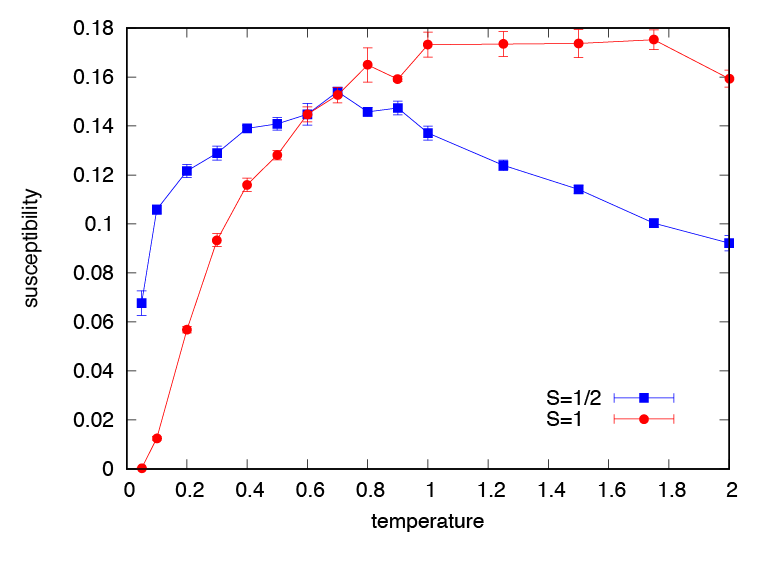
Fig. 3.1 Temperature v.s. susceptibility curves for \(S=1/2\) (blue) and \(S=1\) (red) antiferromagnetic Heisenberg chain.