Input files for Standard mode
An example of input file for the standard mode is shown below:
W = 2
L = 4
model = "spin"

lattice = "triangular lattice"
//mu = 1.0
// t = -1.0
// t' = -0.5
// U = 8.0
//V = 4.0
//V'=2.0
J = -1.0
J'=-0.5
// ncond = 8
Basic rules for input files
In each line, there is a set of a keyword (before an “
=”) and a parameter(after an “=”); they are separated by “=”.You can describe keywords in a random order.
Empty lines and lines beginning in a “
//”(comment outs) are skipped.Upper- and lowercase are not distinguished. Double quotes and blanks are ignored.
There are three kinds of parameters.
Parameters that must be specified (if not,
vmcdry.outwill stop with error messages),Parameters that is not necessary be specified (if not, default values are used),
Parameters that must not be specified (if specified,
vmcdry.outwill stop with error messages).
An example of 3 is transfer \(t\) for the Heisenberg spin system. If you choose “model=spin”, you should not specify “\(t\)”.
We explain each keywords as follows:
Parameters about the kind of a calculation
modelType : String (Choose from
"Fermion Hubbard","Spin","Kondo Lattice","Fermion HubbardGC","SpinGC","Kondo LatticeGC") [1]Description : The target model is specified with this parameter;
"Fermion Hubbard"denotes the canonical ensemble of the Fermion in the Hubbard model(1)¶\[\begin{aligned} H = -\mu \sum_{i \sigma} c^\dagger_{i \sigma} c_{i \sigma} - \sum_{i \neq j \sigma} t_{i j} c^\dagger_{i \sigma} c_{j \sigma} + \sum_{i} U n_{i \uparrow} n_{i \downarrow} + \sum_{i \neq j} V_{i j} n_{i} n_{j}, \end{aligned}\]"Spin"denotes canonical ensemble in the Spin model( \(\{\sigma_1, \sigma_2\}={x, y, z}\))(2)¶\[\begin{split}\begin{aligned} H &= -h \sum_{i} S_{i z} - \Gamma \sum_{i} S_{i x} + D \sum_{i} S_{i z} S_{i z} \nonumber \\ &+ \sum_{i j, \sigma_1}J_{i j \sigma_1} S_{i \sigma_1} S_{j \sigma_1}+ \sum_{i j, \sigma_1 \neq \sigma_2} J_{i j \sigma_1 \sigma_2} S_{i \sigma_1} S_{j \sigma_2} , \end{aligned}\end{split}\]"Kondo Lattice"denotes canonical ensemble in the Kondo lattice model(3)¶\[\begin{aligned} H = - \mu \sum_{i \sigma} c^\dagger_{i \sigma} c_{i \sigma} - t \sum_{\langle i j \rangle \sigma} c^\dagger_{i \sigma} c_{j \sigma} + \frac{J}{2} \sum_{i} \left\{ S_{i}^{+} c_{i \downarrow}^\dagger c_{i \uparrow} + S_{i}^{-} c_{i \uparrow}^\dagger c_{i \downarrow} + S_{i z} (n_{i \uparrow} - n_{i \downarrow}) \right\}. \end{aligned}\]"Fermion HubbardGC","SpinGC", and"Kondo LatticeGC"indicate the \(S_z\)-unconserved Fermion in the Hubbard model [Eqn. (1) ], the \(S_z\)-unconserved Spin model [Eqn. (2) ], and the \(S_z\)-unconserved Kondo lattice model [Eqn. (3) ], respectively. Note: Although these flags has a word “GC”(=grandcanonical), the number of electrons are conserved in these system.The t-J mode is controlled by
NExUpdatePathinmodpara.def(4: spin hopping,5: exchange/spin-hopping mix). At present, Standard mode does not provide a dedicatedmodelkeyword for t-J. The current t-J update paths do not supportBackFloworLocSpin. Since double occupancy is excluded, the input must satisfyncond <= Nsite.latticeType : String (Choose from
"Chain Lattice","Square Lattice","Triangular Lattice","Honeycomb Lattice","Kagome","Ladder")Description : The lattice shape is specified with this parameter; above words denote the one dimensional chain lattice (Fig. 2 (a)), the two dimensional square lattice (Fig. 2 (b)), the two dimensional triangular lattice (Fig. 2 (c)), the two dimensional anisotropic honeycomb lattice (Fig. 3 ), the Kagome Lattice(Fig. 4 ), and the ladder lattice (Fig. 5 ), respectively.
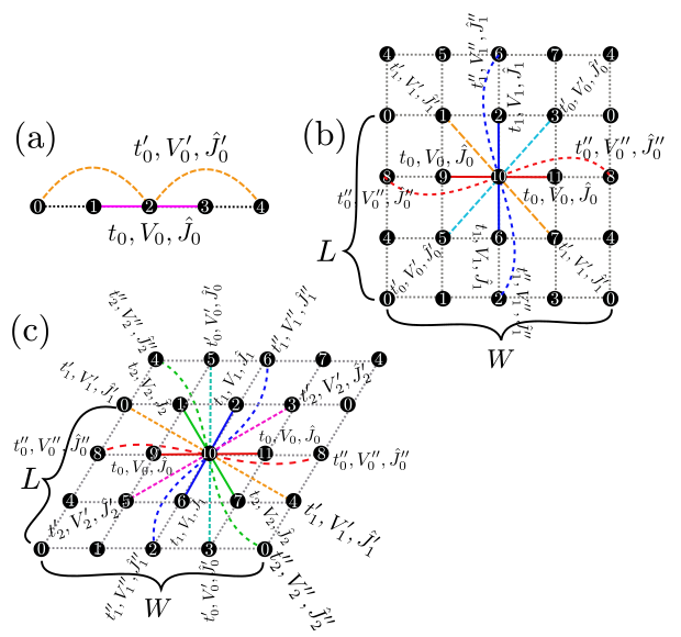
Figure 2: Schematic illustration of (a) one dimensional chain lattice, (b) two dimensional square lattice, and (c) two dimensional triangular lattice. They have \(t\), \(V\), and \(J\) as a nearest neighbor hopping, an offsite Coulomb integral, and a spin-coupling constant, respectively (magenta solid lines); They also have \(t'\), \(V'\), and \(J'\) as a next nearest neighbor hopping, offsite Coulomb integral, and spin-coupling constant, respectively (green dashed line).
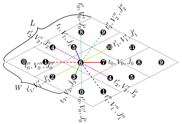
Figure 3: Schematic illustration of the anisotropic honeycomb lattice. The first/second/third nearest neighbor hopping integral, spin coupling, and offsite Coulomb integral depend on the bond direction.
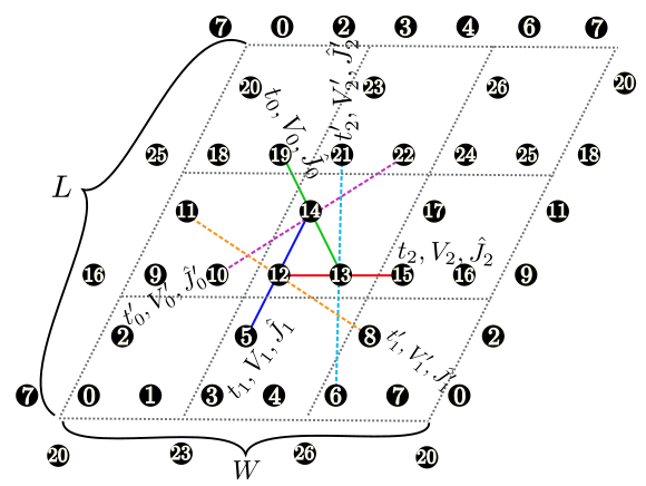
Figure 4: Schematic illustration of the Kagome lattice.
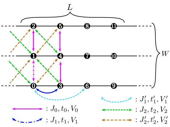
Figure 5: Schematic illustration of the ladder lattice.
Parameters for the lattice
Chain lattice
Fig. 2 (a)
LType : Integer
Description : The length of the chain is specified with this parameter.
Ladder lattice
Fig. 5
LType : Integer
Description : The length of the ladder is specified with this parameter.
WType : Integer
Description : The number of the ladder is specified with this parameter.
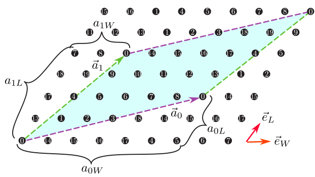
Figure 6: The shape of the numerical cell when \({\vec a}_0 = (6, 2), {\vec a}_1 = (2, 4)\) in the triangular lattice. The region surrounded by \({\vec a}_0\) (Magenta dashed arrow) and \({\vec a}_1\) (Green dashed arrow) becomes the cell to be calculated (20 sites).
Square lattice , Triangular lattice, Honeycomb lattice, Kagome lattice
Square lattice [Fig. 2 (b)], Triangular lattice[Fig. 2 (c)], Honeycomb lattice(Fig. 3 ), Kagome lattice(Fig. 4 )
In these lattices, we can specify the shape of the numerical cell by using the following two methods.
W,LType : Integer
Description : The alignment of original unit cells (dashed black lines in Figs. 2 - 4 ) is specified with these parameter.
a0W,a0L,a1W,a1LType : Integer
Description : We can specify two vectors (\({\vec a}_0, {\vec a}_1\)) that surrounds the numerical cell (Fig. 6 ). These vectors should be specified in the Fractional coordinate.
If we use both of these method, vmcdry.out stops.
We can check the shape of the numerical cell by using a file
lattice.gp (only for square, trianguler, honeycomb, and kagome
lattice) which is written in the Standard mode. This file can be read by
gnuplot as follows:
$ gnuplot lattice.gp
Sublattice
By using the following parameters, we can force the pair-orbital symmetrical to the translation of the sublattice.
a0Wsub,a0Lsub,a1Wsub,a1Lsub,Wsub,LsubType : Positive integer. In the default setting,
a0Wsub=a0W,a0Lsub=a0L,a1Wsub=a1W,a1Lsub=a1L,Wsub=W, andLsub=L. Namely, there is no sublattice.Description : We can specify these parameter as we specify
a0W,a0L,a1W,a1L,W,L. If the sublattice is incommensurate with the original lattice,vmcdry.outstops.
Parameters for the Hamiltonian
A default value is set as \(0\) unless a specific value is not defined in a description. Table [table_interactions] shows the parameters for each models. In the case of a complex type, a file format is “ a real part, an imaginary part “ while in the case of a real type, only “ a real part “.
Local terms
muType : Real
Description : (Hubbard and Kondo lattice model) The chemical potential \(\mu\) (including the site potential) is specified with this parameter.
UType : Real
Description : (Hubbard and Kondo lattice model) The onsite Coulomb integral \(U\) is specified with this parameter.
Jx,Jy,Jz,Jxy,Jyx,Jxz,Jzx,Jyz,JzyType : Real
Description : (Kondo lattice model) The spin-coupling constant between the valence and the local electrons is specified with this parameter. If the exchange coupling
Jis specified in the input file, instead ofJx, Jy, Jz, the diagonal exchange couplings,Jx, Jy, Jz, are set asJx = Jy = Jz = J. When both the set of exchange couplings (Jx,Jy,Jz) and the exchange couplingJare specified in the input file,vmcdry.outwill stop.h,Gamma,DType : Real
Description : (Spin model) The longitudinal magnetic field, transverse magnetic field, and the single-site anisotropy parameter are specified with these parameters. The single-site anisotropy parameter is not available for
model=SpinGCBoost.
The non-local terms described below should be specified in different
ways depending on the lattice structure: For lattice=Ladder, the
non-local terms are specified in the different way from
lattice=Chain Lattice, Square Lattice, Triangular Lattice,
Honeycomb Lattice, Kagome. Below, the available parameters for
each lattice are shown in Table [table_interactions].
Interactions |
1D chain |
2D square |
2D triangular |
Honeycomb |
Kagome |
Ladder |
|---|---|---|---|---|---|---|
|
OK |
OK |
OK |
OK |
OK |
NG |
|
OK |
OK |
OK |
OK |
OK |
OK |
|
NG |
OK |
OK |
OK |
OK |
OK |
|
NG |
NG |
OK |
OK |
OK |
OK |
|
OK |
OK |
OK |
OK |
OK |
NG |
|
OK |
OK |
OK |
OK |
OK |
NG |
|
NG |
OK |
OK |
OK |
OK |
OK |
|
NG |
NG |
OK |
OK |
OK |
OK |
|
OK |
OK |
OK |
OK |
NG |
NG |
|
OK |
OK |
OK |
OK |
NG |
NG |
|
NG |
OK |
OK |
OK |
NG |
NG |
|
NG |
NG |
OK |
OK |
NG |
NG |
Table: Interactions for each models defined in an input file. We can define spin couplings as matrix format.
Non-local terms for Ladder lattice
Fig. 5
t0,t1,t1',t2,t2'Type : Complex
Description : (Hubbard and Kondo lattice model) Hopping integrals in the ladder lattice (See Fig. 5 ) is specified with this parameter.
V0,V1,V1',V2,V2'Type : Real
Description : (Hubbard and Kondo lattice model) Offsite Coulomb integrals on the ladder lattice (Fig. 3 are specified with these parameters.
J0x,J0y,J0z,J0xy,J0yx,J0xz,J0zx,J0yz,J0zyJ1x,J1y,J1z,J1xy,J1yx,J1xz,J1zx,J1yz,J1zyJ1'x,J1'y,J1'z,J1'xy,J1'yx,J1'xz,J1'zx,J1'yz,J1'zyJ2x,J2y,J2z,J2xy,J2yx,J2xz,J2zx,J2yz,J2zyJ2'x,J2'y,J2'z,J2'xy,J2'yx,J2'xz,J2'zx,J2'yz,J2'zyType : Real
Description : (Spin model) Spin-coupling constants in the ladder lattice (See Fig. 5 ) are specified with these parameter. If the simplified parameter
J0is specified in the input file instead of the diagonal couplings,J0x, J0y, J0z, these diagonal couplings are set asJ0x = J0y = J0z = J0. If bothJ0and the set of the couplings (J0x, J0y, J0z) are specified,vmcdry.outwill stop. The above rules are also valid for the simplified parameters,J1,J1',J2, andJ2'.
Non-local terms for other than Ladder
t,t0,t1,t2Type : Complex
Description : (Hubbard and Kondo lattice model) The nearest neighbor hoppings for each direction (see fig_chap04_1_lattice
fig_chap04_1_lattice- fig_kagomefig_kagome) are specified with these parameters. If there is no bond dependence of the hoppings, the simplified parametertis available to specifyt0,t1, andt2ast0 = t1 = t2 = t. If bothtand the set of the hoppings (t0,t1,t2) are specified, the program will stop.t',t0',t1',t2'Type : Complex
Description : (Hubbard and Kondo lattice model) The second nearest neighbor hoppings for each direction (see fig_chap04_1_lattice
fig_chap04_1_lattice- fig_kagomefig_kagome) are specified with these parameter. If there is no bond dependence of the hoppings, the simplified parametert'is available to specifyt0',t1', andt2'ast0' = t1' = t2' = t'. If botht'and the set of the hoppings (t0',t1',t2') are specified, the program will stop.t'',t0'',t1'',t2''Type : Complex
Description : (Hubbard and Kondo lattice model) The third nearest neighbor hoppings for each direction (see fig_chap04_1_lattice
fig_chap04_1_lattice- fig_kagomefig_kagome) are specified with these parameter. If there is no bond dependence of the hoppings, the simplified parametert''is available to specifyt0'',t1'', andt2''ast0'' = t1'' = t2'' = t''. If botht''and the set of the hoppings (t0'',t1'',t2'') are specified, the program will stop.V,V0,V1,V2Type : Real
Description : (Hubbard and Kondo lattice model) The nearest neighbor offsite Coulomb integrals \(V\) for each direction (see fig_chap04_1_lattice
fig_chap04_1_lattice- fig_kagomefig_kagome) are specified with these parameters. If there is no bond dependence of the offsite Coulomb integrals, the simplified parameterVis available to specifyV0,V1, andV2asV0 = V1 = V2 = V. If bothVand the set of the Coulomb integrals (V0,V1,V2) are specified, the program will stop.V',V0',V1',V2'Type : Real
Description : (Hubbard and Kondo lattice model) The second nearest neighbor-offsite Coulomb integrals \(V'\) for each direction (see fig_chap04_1_lattice
fig_chap04_1_lattice- fig_kagomefig_kagome) are specified with this parameter. If there is no bond dependence of the offsite Coulomb integrals, the simplified parameterV'is available to specifyV0',V1', andV2'asV0' = V1' = V2' = V'. If bothV'and the set of the Coulomb integrals (V0',V1',V2') are specified, the program will stop.V'',V0'',V1'',V2''Type : Real
Description : (Hubbard and Kondo lattice model) The third nearest neighbor-offsite Coulomb integrals \(V'\) for each direction (see fig_chap04_1_lattice
fig_chap04_1_lattice- fig_kagomefig_kagome) are specified with this parameter. If there is no bond dependence of the offsite Coulomb integrals, the simplified parameterV''is available to specifyV0'',V1'', andV2''asV0'' = V1'' = V2'' = V''. If bothV''and the set of the Coulomb integrals (V0'',V1'',V2'') are specified, the program will stop.J0x,J0y,J0z,J0xy,J0yx,J0xz,J0zx,J0yz,J0zyJ1x,J1y,J1z,J1xy,J1yx,J1xz,J1zx,J1yz,J1zyJ2x,J2y,J2z,J2xy,J2yx,J2xz,J2zx,J2yz,J2zyType : Real
Description : (Spin model) Nearest-neighbor exchange couplings for each direction are specified with thees parameters. If the simplified parameter
J0is specified, instead ofJ0x, J0y, J0z, the exchange couplings,J0x, J0y, J0z, are set asJ0x = J0y = J0z = J0. If bothJ0and the set of the exchange couplings (J0x, J0y, J0z) are specified,vmcdry.outwill stop. The above rules are valid forJ1andJ2.If there is no bond dependence of the nearest-neighbor exchange couplings, the simplified parameters,
Jx,Jy,Jz,Jxy,Jyx,Jxz,Jzx,Jyz,Jzy, are available to specify the exchange couplings for every bond asJ0x = J1x = J2x = Jx. If any simplified parameter (Jx\(\sim\)Jzy) is specified in addition to its counter parts (J0x\(\sim\)J2zy),vmcdry.outwill stop. Below, examples of parameter sets for nearest-neighbor exchange couplings are shown.If there are no bond-dependent, no anisotropic and offdiagonal exchange couplings (such as \(J_{x y}\)), please specify
Jin the input file.If there are no bond-dependent and offdiagonal exchange couplings but are anisotropic couplings, please specify the non-zero couplings in the diagonal parameters,
Jx, Jy, Jz.If there are no bond-dependent exchange couplings but are anisotropic and offdiagonal exchange couplings, please specify the non-zero couplings in the nine parameters,
Jx, Jy, Jz, Jxy, Jyz, Jxz, Jyx, Jzy, Jzx.If there are no anisotropic and offdiagonal exchange couplings, but are bond-dependent couplings, please specify the non-zero couplings in the three parameters,
J0, J1, J2.If there are no anisotropic exchange couplings, but are bond-dependent and offdiagonal couplings, please specify the non-zero couplings in the nine parameters,
J0x, J0y, J0z, J1x, J1y, J1z, J2x, J2y, J2z.If there are bond-dependent, anisotropic and offdiagonal exchange couplings, please specify the non-zero couplings in the twenty-seven parameters from
J0xtoJ2zy.
J'x,J'y,J'z,J'xy,J'yx,J'xz,J'zx,J'yz,J'zyJ0'x,J0'y,J0'z,J0'xy,J0'yx,J0'xz,J0'zx,J0'yz,J0'zyJ1'x,J1'y,J1'z,J1'xy,J1'yx,J1'xz,J1'zx,J1'yz,J1'zyJ2'x,J2'y,J2'z,J2'xy,J2'yx,J2'xz,J2'zx,J2'yz,J2'zyType : Real
Description : (Spin model) The second nearest neighbor exchange couplings are specified. However, for
lattice = Honeycomb Latticeandlattice = Kagomewithmodel=SpinGCCMA, the second nearest neighbor exchange couplings are not available in the \(Standard\) mode. If the simplified parameterJ'is specified, instead ofJ'x, J'y, J'z, the exchange couplings are set asJ'x = J'y = J'z = J'. If bothJ'and the set of the couplings (J'x, J'y, J'z) are specified, the program will stop.J''x,J''y,J''z,J''xy,J''yx,J''xz,J''zx,J''yz,J''zyJ0''x,J0''y,J0''z,J0''xy,J0''yx,J0''xz,J0''zx,J0''yz,J0''zyJ1''x,J1''y,J1''z,J1''xy,J1''yx,J1''xz,J1''zx,J1''yz,J1''zyJ2''x,J2''y,J2''z,J2''xy,J2''yx,J2''xz,J2''zx,J2''yz,J2''zyType : Real
Description : (Spin model) The third nearest neighbor exchange couplings are specified. However, for
lattice = Honeycomb Latticeandlattice = Kagomewithmodel=SpinGCCMA, the third nearest neighbor exchange couplings are not available in the \(Standard\) mode. If the simplified parameterJ''is specified, instead ofJ''x, J''y, J''z, the exchange couplings are set asJ''x = J''y = J''z = J''. If bothJ''and the set of the couplings (J''x, J''y, J''z) are specified, the program will stop.phase0,phase1Type : Double (
0.0as defaults)Description : We can specify the phase for the hopping through the cell boundary with these parameter (unit: degree). These factors for the \(\vec{a}_0\) direction and the \(\vec{a}_1\) direction can be specified independently. For the one-dimensional system, only
phase0can be used. For example, a fopping from \(i\)-th site to \(j\)-th site through the cell boundary with the positive direction becomes as\[\begin{aligned} \exp(i \times {\rm phase0}\times\pi/180) \times t {\hat c}_{j \sigma}^\dagger {\hat c}_{i \sigma} + \exp(-i \times {\rm phase0}\times\pi/180) \times t^* {\hat c}_{i \sigma}^\dagger {\hat c}_{j \sigma} \end{aligned}\]
Parameters for the numerical condition
ncondType : int-type (must be specified)
Description : The number of itinerant electrons. It is the sum of the \(\uparrow\) and \(\downarrow\) electrons.
NVMCCalModeType : int-type (default value: 0)
Description : [0] Optimization of variational parameters, [1] Calculation of one body and two body Green’s functions.
NDataIdxStartType : int-type (default value: 1)
Description : An integer for numbering of output files. For
NVMCCalMode= 0 ,NDataIdxStartis added at the end of the output files. ForNVMCCalMode= 1, the files are outputted with the number fromNDataIdxStarttoNDataIdxStart+NDataQtySmp-1.NDataQtySmpType : int-type (default value: 1)
Description : The set number for outputted files (only used for
NVMCCalMode= 1).NSPGaussLegType : int-type (Positive integer, default value is 8 for
2Sz=0)Description : The mesh number for the Gauss-legendre quadrature about \(\beta\) integration (\(S_y\) rotation) for the spin quantum-number projection in actual numerical calculation.
NSPStotType : int-type ( greater equal 0, default value is 0 for
2Sz=0)Description : The total spin quantum-number.
2SzType : int-type ( greater equal 0, default value is 0)
Description : The spin quantum-number \(S_z\).
NMPTransType : int-type (Positive integer. Default
1)Description : The number of the momentum and lattice translational quantum-number projection. In the case of not to apply the projection, this value must be set as 1.
NSROptItrStepType : int-type (Positive integer, default value: 1000)
Description : The whole step number to optimize variational parameters by SR method. Only used for
NVMCCalMode=0.NSROptItrSmpType : int-type (Positive integer, default value:
NSROptItrStep/10)Description : In the
NSROptItrStepstep, the average values of the each variational parameters at theNSROptItrStepstep are adopted as the optimized values. Only used forNVMCCalMode=0.DSROptRedCutType : double-type (default value: 0.001)
Description : The stabilized factor for the SR method by truncation of redundant directions corresponding to \(\varepsilon_{\rm wf}\) in the ref. [Tahara2008 ].
DSROptStaDelType : double-type (default value: 0.02)
Description : The stabilized factor for the SR method by modifying diagonal elements in the overwrap matrix corresponding to \(\varepsilon\) in the ref. [Tahara2008 ].
DSROptStepDtType : double-type (default value: 0.02)
Description : The time step using in the SR method.
NVMCWarmUpType : int-type (Positive integer, default value: 10)
Description : Idling number for the Malkov chain Montecarlo Methods.
NVMCIntervalType : int-type (Positive integer, default value: 1)
Description : The interval step between samples. The local update will be performed
Nsite×NVMCIntervaltimes.NVMCSampleType : int-type (Positive integer, default value: 1000)
Description : The sample numbers to calculate the expected values.
NExUpdatePathType : int-type (Non-negative integer)
Description : The option for local updates. The choices are 0: hopping, 1: exchange or hopping, 2: exchange, 3: KondoGC update (hopping or exchange/local-spin-flip), 4: t-J spin hopping, 5: t-J update (exchange or spin hopping), and 6: doublon-only sampling by pair hopping. In Standard mode, this value is assigned automatically from
model. To use t-J mode, setNExUpdatePath=4or5inmodpara.def. The t-J choices do not supportBackFloworLocSpin. Since double occupancy is excluded, the input must satisfyncond <= Nsite. To useNExUpdatePath=6, set it inmodpara.defafter generating the expert-mode files. This mode restricts each site to empty or doublon states, \((n_{\uparrow}, n_{\downarrow})=(0,0)\) or \((1,1)\), requires0 < Ne < Nsiteand an anti-parallel-spinOrbitalinput, and currently does not supportLocSpin,BackFlow, RBM, orOrbitalGeneral/FSZ inputs.RndSeedType : int-type (default value: 123456789)
Description : The initial seed of generating random number. For MPI parallelization, the initial seeds are given by
RndSeed+my rank+1 at each ranks.NSplitSizeType : int-type (Positive integer, default value: 1)
Description : The number of processes of MPI parallelization.
NStoreType : int-type (0 or 1, default value: 1)
Description : The option of applying matrix-matrix product to calculate expected values \(\langle O_k O_l \rangle\) (0: off, 1: on). This speeds up calculation but increases the amount of memory usage from \(O(N_\text{p}^2)\) to \(O(N_\text{p}^2) + O(N_\text{p}N_\text{MCS})\), where \(N_\text{p}\) is the number of the variational parameters and \(N_\text{MCS}\) is the number of Monte Carlo sampling.
NSRCGType : int-type (0 or 1, default value: 0)
Description : The option of solving \(Sx=g\) in the SR method without constructing \(S\) matrix [NeuscammanUmrigarChan ]. (0: off, 1: on). This reduces the amount of memory usage from \(O(N_\text{p}^2) + O(N_\text{p}N_\text{MCS})\) to \(O(N_\text{p}) + O(N_\text{p}N_\text{MCS})\) when \(N_\text{p} > N_\text{MCS}\).
ComplexTypeType : int-type (
0or1. Default value is0for the \(S_z\)-conserved system and1for the \(S_z\)-unconserved system.)Description : If it is
0, only the real part of the variational parameters are optimized. And the real and the imaginary part of them are optimized if this parameter is1.OutputModeType : Choose from
"none","correlation", and"full"(correlationas a default)Description : Indices of correlation functions are specified with this keyword.
"none"indicates correlation functions will not calculated. Whenoutputmode="correlation", the correlation function supported by the utilityfourieris computed. For more details, see the document indoc/fourier/. If"full"is selected, \(\langle c_{i \sigma}^{\dagger}c_{j \sigma'} \rangle\) is computed at all \(i, j, \sigma, \sigma'\), and \(\langle c_{i_1 \sigma}^{\dagger}c_{i_2 \sigma} c_{i_3 \sigma'}^{\dagger}c_{i_4 \sigma'} \rangle\) is computed at all \(i_1, i_2, i_3, i_4, \sigma, \sigma'\).In spin system, indices are specified as those on the Bogoliubov representation (See [sec_bogoliubov_rep]).
CDataFileHeadType : string-type (default :
"zvo")Description : A header for output files. For example, the output filename for one body Green’s function becomes “ xxx_cisajs_yyy.dat” (xxx are characters set by
CDataFileHeadand yyy are numbers given by numbers fromNDataIdxStarttoNDataIdxStart+NDataQtySmp).CParaFileHeadType : string-type (default :
"zqp")Description : A header for output files of the optimized variational parameters. For example, the optimized variational parameters are outputted as zzz_opt_yyy.dat (zzz are characters set by
CParaFileHeadand yyy are numbers given by numbers fromNDataIdxStarttoNDataIdxStart+NDataQtySmp-1).