Search for the Neel temperature

In this tutorial, we search for the Neel temperature of the single band Hubbard model on the square lattice. To this end, we calculate the susceptibility at different temperatures and find the temperature where the inverse susceptibility becomes zero. Sample files for this tutorial are available at examples/square_bse_TNeel.

Model

The model parameters such as \(U\) are the same as in the previous tutorial. The common part of the input file of DCore is dmft_square.in:

[model]
seedname = square
lattice = wannier90
norb = 1
nelec = 1.0
t = -1.0
kanamori = [(8.0, 0.0, 0.0)]
nk0 = 32
nk1 = 32
nk2 = 1

#[mpi]
#command = "mpirun -n #"

[impurity_solver]
name = pomerol
exec_path{str} = pomerol2dcore
n_bath{int} = 0
fit_gtol{float} = 1e-6

[control]
max_step = 10
sigma_mix = 1.0
converge_tol = 1e-5
n_converge = 3

[bse]
num_wb = 1
num_wf = 20
X0q_qpoints_saved = q_path.dat

[system]
# T = 0.5
n_iw = 1024
mu = 4.0
fix_mu = True

Compared to the previous example, we move the [system] section to the bottom of the file and remove the T parameter from it. This is because we will vary the temperature by adding different T parameters when running the script.

Workflow and results

A script file, run.sh, which is shown below:

#!/bin/bash

if [ -z "$NPROCS" ]; then
  echo "NPROCS (number of MPI processes) is not defined"
  echo "Example: $ NPROCS=1 sh ./run.sh"
  exit 1
fi

echo "NPROCS = $NPROCS"

set -uex

ROOTDIR=$(pwd)
ini=dmft_square.in

# (1) Perform preprocess
rm -f square.h5
dcore_pre $ini 1>dcore_pre.log 2>dcore_pre.err
gen_qpath.py $ini qpath.in
rm -f chi.dat
echo "# T chi" > chi.dat

# (2) Get the momentum of M point as Q_M (e.g., 16.16.00)
# Tips: In AWK, $(NF) means the last field of the line.
Q_M=$(awk '$(NF)=="M" {print $2}' < q_path.dat)

for T in 0.4 0.5 0.6 0.7 0.8 0.9 1.0; do
  echo "T = $T"
  cd "$ROOTDIR"

  # (3) Create a directory for each temperature, copy necessary files, and add T to the input file
  # NOTE: remove the directory and its contents if it already exists
  rm -rf T_$T
  mkdir -p T_$T
  for f in dmft_square.in square.h5 square_hr.dat q_path.dat bse.in; do
    cp $f T_$T
  done
  echo "T = ${T}" >> T_$T/$ini
  cd T_$T

  # (4) calculate susceptibilities by BSE
  dcore $ini --np $NPROCS 1>dcore.log 2>dcore.err
  dcore_check $ini 1>dcore_check.log 2>dcore_check.err
  dcore_chiq.py $ini --np $NPROCS 1>dcore_chiq.log 2>dcore_chiq.err
  mpirun -np $NPROCS chiq_main.py bse.in 1>chiq_main.log 2>chiq_main.err
  chiq_post.py bse.in 1>chiq_post.log 2>chiq_post.err

  # (5) get chi at Q_M and save to chi.dat
  chi=$(awk -v Q="${Q_M}" '$2==Q {print $3}' < bse/chi_q_eigen.dat)
  echo "$T $chi" >> ../chi.dat

  # Plot BSE results
  (
    cd bse
    plot_chiq_path.py ../q_path.dat chi_q_eigen.dat
  )

  cd "$ROOTDIR"
done

# Plot the inverse susceptibility
gnuplot plot_chiinv.plt

echo "Finished successfully"

To run the script, you need to set the NPROCS (number of MPI processes). For example, NPROCS=1 sh run.sh.

1. Perform preprocess

• square.h5 and q_path.dat are common files for all temperatures.

• chi.dat is an empty file to store the susceptibility at Q_M for each temperature.

2. Get the momentum of M point as Q_M.

• In q_path.dat, the second field of the line with M indicates the momentum of M point:

  0 16.16.00   1.20711 M
  

3. Create a directory for each temperature, copy necessary files and add T to the input file.

• Since we moved the [system] section to the bottom, we can simply append T = $T to the file.

4. Calculate the susceptibility by ChiQ.

• The procedure is the same as in the previous tutorial.

• bse.in is a little bit different from the previous example. We will describe it in the next section.

5. Get the susceptibility at Q_M and save to chi.dat.

• Find the line with the second field equal to Q_M in bse/chi_q_eigen.dat and get the third field.

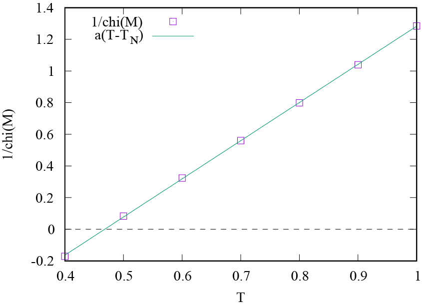
After running the script, we obtain chi.dat storing pairs of \(T\) and \(\chi(q_{\boldsymbol{M}})\).

By fitting the inverse susceptibility \(1/\chi(q_{\boldsymbol{M}})\) by a function \(1/\chi = a(T-T_\text{N})\), we estimate the Neel temperature \(T_\text{N} = 0.467(1)\).

Sorting the eigenvalues

In this example, \(\chi(\boldsymbol{q})\) has four modes; three of them are degenerate over the whole momentum space and the other is far away from them. The degenerated modes diverge at M point at the Neel temperature as follows. As temperature approaches the Neel temperature from above, the susceptibility \(\chi(q_{\boldsymbol{M}})\) grows and finally diverges. Below the Neel temperature, \(\chi(q_{\boldsymbol{M}})\) obtained by solving BSE becomes negative. In other words, the inverse susceptibility \(1/\chi(q_{\boldsymbol{M}})\) becomes zero from above at the Neel temperature, and becomes negative below the Neel temperature. The following figures show \(1/\chi(\boldsymbol{q})\) for temperatures \(T = 0.5 > T_\text{Neel}\) and \(T = 0.4 < T_\text{Neel}\).

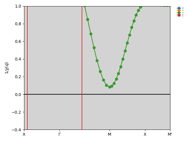
\(1/\chi(\boldsymbol{q})\) for \(T = 0.5 > T_\text{Neel}\).

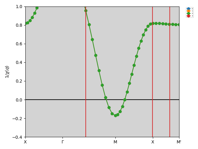
\(1/\chi(\boldsymbol{q})\) for \(T = 0.4 < T_\text{Neel}\).

We need to sort the eigenvalues properly to pursue the diverging modes. By setting order = overlap in the [chiq_post] section, the eigenvalues are sorted based on the overlap with the eigenvector at the previous momentum (at the first momentum, X in this case, the eigenvalues are sorted in descending order). With this change, the bse.in file is as follows:

[chiq_common]
input = "dmft_bse.h5"
output = "dmft_bse.out.h5"
type = ["chi0","bse"]
omega_q = "q_path.dat"

[chiq_main]
work_dir = "work/chiq"

[chiq_post]
output_dir = "bse"
mode = ["eigen"]
order = "overlap"