Intersite interactions

In this tutorial, we calculate the intersite interactions of the single band Hubbard model on the square lattice. For details of the intersite interactions, see Intersite interactions in Algorithms. Sample files for this tutorial are available at examples/square_Ir.

Model

The model parameters such as \(U\) are the same as in the previous tutorial. The input file of DCore is dmft_square.in:

[model]
seedname = square
lattice = wannier90
norb = 1
nelec = 1.0
t = -1.0
kanamori = [(8.0, 0.0, 0.0)]
nk0 = 32
nk1 = 32
nk2 = 1

#[mpi]
#command = "mpirun -n #"

[system]
T = 0.5
n_iw = 1024
mu = 4.0
fix_mu = True

[impurity_solver]
name = pomerol
exec_path{str} = pomerol2dcore
n_bath{int} = 0
fit_gtol{float} = 1e-6

[control]
max_step = 10
sigma_mix = 1.0
converge_tol = 1e-5
n_converge = 3

[bse]
num_wb = 1
num_wf = 20
X0q_qpoints_saved = "q_fbz.dat"

Compared to the previous example, the X0q_qpoints_saved parameter in the [bse] section is set to q_fbz.dat from q_path.dat. This is because we need to calculate the intersite interactions for all the points in the BZ (fbz means full Brillouin zone) in order to perform FFT from the momentum space to the real space.

Workflow

Calculation of susceptibility \(\chi(q)\)

First, we perform the DMFT calculation as usual.

dcore_pre dmft_square.in
dcore --np 4 dmft_square.in

Before running dcore_chiq.py, we need to prepare the q_fbz.dat file by using the gen_allq.py script.

gen_allq.py dmft_square.in

Run dcore_chiq.py and chiq_main.py to calculate the susceptibility in the momentum space, \(\chi(q)\) and \(\chi_\text{loc}(q)\).

dcore_chiq.py --np 4 dmft_square.in
mpiexec -np 4 chiq_main.py bse.in

The input file of ChiQ tools, bse.in, is also the same as in the previous tutorial:

[chiq_common]
input = "dmft_bse.h5"
output = "dmft_bse.out.h5"
type = ["chi0", "bse"]  # "chi0", "bse", "scl", "rpa", "rrpa"
omega_q = "q_fbz.dat"

[chiq_main]
work_dir = "work/chiq"
# num_wf = 20  # If not specified, the value is determined from X_loc

[chiq_post]
output_dir = "bse"
mode = ["eigen"]  # "matrix_element", "eigen", "linear_combination"

# for mode="eigen"
#vector = true  # output eigenvectors
order = "file"  # "descend" (default), "overlap", "file"
order_file = "eigenvec.in"  # for order="file"

# for mode="linear_combination"
# coefs_file = "/path/to/coefs.in"

The only difference is that the q_fbz.dat file is used instead of q_path.dat in omega_q parameter in the [chiq_common] section.

Calculation of intersite interactions \(I(q)\) and \(I(r)\)

Once these susceptibilities are calculated, we can run calc_Iq.py to calculate the intersite interactions in the momentum space, \(I(q)\).

calc_Iq.py -f dmft_bse.out.h5 --remove 1

-f is used to specify the HDF5 file, which is the output file of chiq_main.py (in this case, dmft_bse.out.h5). --remove specifies the number of the modes to be removed to stabilize the calculation. In this case, we remove one mode with the smallest eigenvalue. The obtained \(I(q)\) is saved in the HDF5 file as dmft_bse.out.h5/bse/output/I_q.

Next, we perform the FFT from the momentum space \(I(q)\) to the real space \(I(r)\) by using chiq_fft.py.

chiq_fft.py -f dmft_bse.out.h5 --input_dname I_q --output_dname I_r dmft_square.in

-f is used to specify the HDF5 file, which is used in calc_Iq.py (in this case, dmft_bse.out.h5). --input_dname is used to specify the name of the dataset in the HDF5 file of \(I(q)\) (in this case, I_q). --output_dname is used to specify the name of the dataset in the HDF5 file of \(I(r)\) (in this case, I_r). In this case, chiq_fft.py reads the \(I(q)\) from dmft_bse.out.h5/bse/output/I_q and writes the \(I(r)\) to dmft_bse.out.h5/bse/output/I_r.

Finally, as in the case of \(\chi(q)\), we need to transform (or diagonalize) \(I(q)\) to \(I(r)\) by using chiq_post.py.

mpiexec --np 4 chiq_post.py bse.in

This also transforms \(I(q)\) and \(I(r)\) in the same way as \(\chi(q)\). The results, I_q_eigen.dat and I_r_eigen.dat, are saved in the directory specified by output_dir parameter in the [chiq_post] section of bse.in (in this case, bse directory). The file format is also the same as in the \(\chi(q)\) case.

Plotting the results

\(I(q)\) can be plotted in the same way as \(\chi(q)\) in the previous tutorial.

First, we prepare a q-path file, q_path.dat:

gen_qpath.py dmft_square.in qpath.in

Then, we plot \(I(q)\) as follows in the bse directory:

plot_chiq_path.py --label ../label2.in --mode=Iq ../q_path.in I_q_eigen.dat

The following figure I_q_eigen_path.pdf is saved.

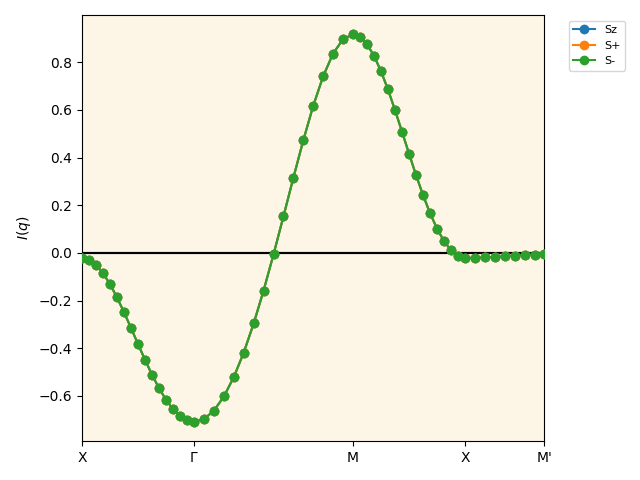
\(I(q)\) calculated by the BSE.

On the other hand, \(I(r)\) can be plotted by using plot_Ir.py. This script plots \(I(r)\) as a function of the distance from the origin. In the bse directory, run the following command:

plot_Ir.py --label ../label2.in I_r_eigen.dat

The following figure I_r_eigen_distance.pdf is saved.

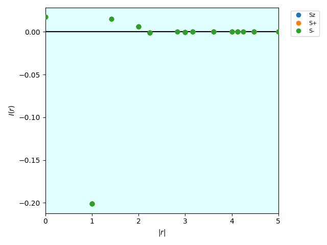
\(I(r)\) calculated by the BSE.