Single band Hubbard model
In this tutorial, we calculate the susceptibility of the single band Hubbard model on the square lattice by using the BSE, RPA, and SCL approximations with the DMFT.
Sample files for this tutorial are available at examples/square_bse (BSE), examples/square_rpa (RPA), and examples/square_scl (SCL).
Model
As the first example, we consider the single band Hubbard model on the \(32 \times 32\) square lattice with the periodic boundary condition,
where \(\varepsilon_{\boldsymbol{k}} = -2t(\cos k_x + \cos k_y)\) is the dispersion relation of the non-interacting electrons with momentum \(\boldsymbol{k}\) and \(t\) is the hopping constant. \(c_{\boldsymbol{k}\sigma}^\dagger\) and \(c_{\boldsymbol{k}\sigma}\) are the creation and annihilation operators of electrons with momentum \(\boldsymbol{k}\) and spin \(\sigma\), respectively, and \(n_{i\sigma} = c_{i\sigma}^\dagger c_{i\sigma}\) is the number operator of electrons with spin \(\sigma\) at site \(i\). The onsite Coulomb interaction strength is denoted by \(U\). We consider the half-filled case with one electron per site. The parameters are set to be \(t = 1.0\) (the unit of energy), \(U = 8.0\). We can fix the chemical potential as \(\mu = U/2 = 4.0\). The temperature is set to be \(T = 0.5\) and the number of Matsubara frequencies is set to be \(N_{\text{freq}} = 1024\). The impurity solver in the DMFT loop is the Hubbard-I (the exact diagonalization with no bath sites). We can safely set the number of DMFT iterations to be \(N_{\text{iter}} = 1\).
DMFT calculation with DCore
To implement this setup, an input file of DCore dmft_square.in is prepared as follows,
[model]
seedname = square
lattice = wannier90
norb = 1
nelec = 1.0
t = -1.0
kanamori = [(8.0, 0.0, 0.0)]
nk0 = 32
nk1 = 32
nk2 = 1

#[mpi]
#command = "mpirun -n #"

[system]
T = 0.5
n_iw = 1024
mu = 4.0
fix_mu = True

[impurity_solver]
name = pomerol
exec_path{str} = pomerol2dcore
n_bath{int} = 0
fit_gtol{float} = 1e-6

[control]
max_step = 1
sigma_mix = 1.0
converge_tol = 1e-5
n_converge = 3

[bse]
num_wb = 1
num_wf = 20
X0q_qpoints_saved = "q_path.dat"
In this example, the Wannier90 format is used to describe the hopping constants (set lattice = wannier90).
Because seed = square, the hopping constants are read from the following file square_hr.dat,
square lattice
1
9
1 1 1 1 1 1 1 1 1
-1 -1 0 1 1   0.0 0.0
-1  0 0 1 1  -1.0 0.0
-1  1 0 1 1   0.0 0.0
 0 -1 0 1 1  -1.0 0.0
 0  0 0 1 1   0.0 0.0
 0  1 0 1 1  -1.0 0.0
 1 -1 0 1 1   0.0 0.0
 1  0 0 1 1  -1.0 0.0
 1  1 0 1 1   0.0 0.0
This file says that the number of the orbitals in the unit cell is 1 and the electrons hop to the nearest neighbors on a square lattice with \(t = 1.0\) (watch out the sign of the hopping constant). For details, see the paper of DCore and the Wannier90 manual.
Before running the DMFT calculation, make sure that pomerol2dcore is installed and in your PATH.
A DMFT calculation is performed with DCore as follows (we will use 4 MPI processes in the following):
dcore_pre dmft_square.in
dcore --np 4 dmft_square.in
After the DMFT loop is finished, the impurity problem is solved again to calculate the bare two-particle Green’s functions \(\hat{X}_0\) and the local two-particle Green’s function \(\hat{X}_\text{loc}\) (see Bethe-Salpeter equation (BSE)).
The number of the fermionic and bosonic Matsubara frequencies \(\omega_n\) and \(\Omega_m\) are specified by the keywords num_wf and num_wb, respectively, in the [bse] section of the input file of DCore (see above).
X0q_qpoints_saved is the file name describing \((\boldsymbol{q}, i\Omega_m)\) points where \(\hat{X}_0\) and \(\hat{X}_\text{loc}\) are calculated.
Generally, a q-path file is used as this file.
To generate the q-path file easily, an utility script gen_qpath.py is available. By using the following symmetry point file qpath.in
# qx qy qz name  (in unit of reciprocal lattice vectors)
1/2 0 0  X
0 0 0  Gamma
1/2 1/2 0  M
1/2 0 0  X
1/4 1/4 0  M'
and the input file of DCore dmft_square.in, the q-path file q_path.dat is generated by the following command
gen_qpath.py dmft_square.in qpath.in
Once the input files are prepared, the following command:
dcore_chiq.py --np 4 dmft_square.in
calculates \(\hat{X}_0\) and \(\hat{X}_\text{loc}\) and writes them to one of the input file of BSE, dmft_bse.h5 .
BSE calculation with ChiQ
The following is the input file of ChiQ bse.in:
[chiq_common]
input = "dmft_bse.h5"
output = "dmft_bse.out.h5"
type = ["chi0", "bse", "rpa", "rrpa"]  # "chi0", "bse", "scl", "rpa", "rrpa"
omega_q = "q_path.dat"

[chiq_main]
work_dir = "work/chiq"
# num_wf = 20  # If not specified, the value is determined from X_loc

[chiq_post]
output_dir = "bse"
mode = ["eigen"]  # "matrix_element", "eigen", "linear_combination"

# for mode="eigen"
vector = true  # output eigenvectors
# order = "file"  # "descend" (default), "overlap", "file"
# order_file = "/path/to/eigenvec.in"  # for order="file"

# for mode="linear_combination"
# coefs_file = "/path/to/coefs.in"
[chiq_common] section is common to all the ChiQ scripts.
The input keyword specifies the HDF5 file including the Green’s functions, which is the output file of dcore_chiq.py.
The output keyword specifies the HDF5 file to store the results of BSE calculation (e.g., the susceptibility).
The type keyword specifies the approximation method in calculating the susceptibility.
The omega_q keyword specifies the q-path file.
The BSE calculation is performed by chiq_main.py. The following command calculates the susceptibility \(\chi_{ijkl}(\boldsymbol{q}, i\Omega_m)\) and writes the result to the file dmft_bse.out.h5 :
mpiexec --np 4 chiq_main.py bse.in
The calculation log from each process is saved in the directory specified by the work_dir keyword in the [chiq_main] section.
Because the number of the spin-orbitals is 2 (up and down spin), the calculated susceptibility at each q-point is represented as \(4 \times 4\) matrix, \(\chi_{ij,kl}\).
To analyze further, we need to diagonalize the susceptibility matrix (see Analyzing the susceptibility).
chiq_post.py is used to calculate the eigenvalues of them.
The parameters are specified by the [chiq_post] section.
The mode keyword specifies how to calculate the eigenvalues. 'eigen' calculates the eigenvalues by diagonalizing the susceptibility matrix.
The following command calculates the eigenvalues and eigenvectors of the susceptibility matrix :
mpiexec --np 4 chiq_post.py bse.in
The result is saved in the text files like chi_q_eigen.dat in the directory specified by the output_dir keyword in the [chiq_post] section.
The eigenvalue files have \(2 + N_\text{eigen}\) columns, where \(N_\text{eigen}\) is the number of the eigenvalues.
The first two columns are the index of the bosonic Matsubara frequency \(m\) of \(\nu_m\) and the index of the q-point \(\boldsymbol{q}\), respectively, as same as the q-path file.
The remaining columns are the eigenvalues.
chi_q_eigen.dat is the file for the BSE calculation.
For the RPA, RRPA, and SCL calculation, the file name is chi_q_rrpa_eigen.dat, chi_q_rrpa_eigen.dat, and chi_q_scl_eigen.dat, respectively.
If you set the vector keyword in the [chiq_post] section to true, the eigenvectors at k-points are also saved in the files like chi_q_eigenvec.00.00.00.dat.
eigenvec_viewer.py helps to analyze the eigenvectors.
For details of the eigenvector file format and the usage of eigenvec_viewer.py, see eigenvec_viewer.
Finally, plot_chiq_path.py plots the eigenvalues *_eigen_path.pdf and their inverse *_eigen_path_inv.pdf along the q-path.
The first argument is the q-path file, and the second argument is the eigenvalue file.
# Make sure that you are in the output directory of chiq_post.py
plot_chiq_path.py ../q_path.dat chi_q_eigen.dat
The following figure is the result of the BSE calculation (chi_q_eigen_path.pdf).
The susceptibility has a sharp peak at the M point, \(\boldsymbol{q} = (\pi, \pi)\), indicating the growth of the antiferromagnetic fluctuations.
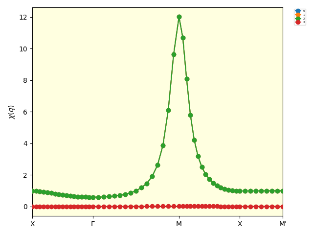
The eigenvalues of the two-body susceptibility calculated by solving the BSE.
Random phase approximation (RPA)
ChiQ also provides the RPA calculation. In the RPA calculation, the interaction is taken into account only via the symmetrized vertex function \(\hat{\gamma}\), not via the self-energy \(\Sigma\). So, the DMFT calculation needs to be solved with the “null” solver, which gives the self-energy \(\Sigma = 0\) (see Random phase approximation (RPA)). The input file of DCore follows:
[model]
seedname = square
lattice = wannier90
norb = 1
nelec = 1.0
t = -1.0
kanamori = [(1.0, 0.0, 0.0)]
nk0 = 32
nk1 = 32
nk2 = 1

#[mpi]
#command = "mpirun -n #"

[system]
T = 0.5
n_iw = 1024
mu = 0.0
#fix_mu = True

[impurity_solver]
name = null

[control]
max_step = 1
# No self-energy iteration is needed for null solver

[bse]
num_wb = 1
num_wf = 20
X0q_qpoints_saved = "q_path.dat"
skip_Xloc = True
Note that the interaction strength \(U\) is set to be one, not eight. This is because the RPA overestimates the Neel temperature, and hence the point \(U=8\) and \(T=0.5\) is the antiferromagnetic phase and too far from the phase transition point. It should also be noted that the chemical potential \(\mu\) is set to be zero, because the DMFT loop is calculated as \(U=0\).
In the input file bse.in, the only difference from the previous calculation is that the type keyword of [chiq_common] section is set to ['chi0', 'rpa'].
[chiq_common]
input = "dmft_bse.h5"
output = "dmft_bse.out.h5"
type = ["chi0", "rpa"]  # "chi0", "bse", "scl", "rpa", "rrpa"
omega_q = "q_path.dat"

[chiq_main]
work_dir = "work/chiq"
# num_wf = 20  # If not specified, the value is determined from X_loc

[chiq_post]
output_dir = "bse"
mode = ["eigen"]  # "matrix_element", "eigen", "linear_combination"

# for mode="eigen"
#vector = true  # output eigenvectors
#order = "file"  # "descend" (default), "overlap", "file"
#order_file = "/path/to/eigenvec.in"  # for order="file"

# for mode="linear_combination"
# coefs_file = "/path/to/coefs.in"
The workflow is the same as the previous calculation.
Note that the names of the output files by the RPA calculation start with chi_q_rpa_.
dcore_pre dmft_square.in
dcore --np 4 dmft_square.in
gen_qpath.py dmft_square.in qpath.in
dcore_chiq.py --np 4 dmft_square.in
mpiexec --np 4 chi_main.py bse.in
mpiexec --np 4 chiq_post.py bse.in
cd bse
plot_chiq_path.py ../q_path.dat chi_q_rpa_eigen.dat
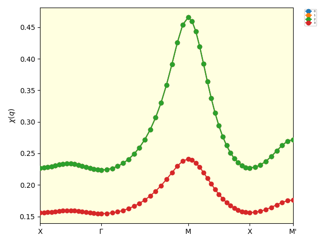
The eigenvalues of the two-body susceptibility calculated by the RPA.
Strong coupling limit formula (SCL)
Finally, ChiQ provides the calculation tool based on the strong coupling limit formula (SCL) (see Strong-coupling limit formula (SCL)). The input file of DCore is the same as the previous BSE calculation.
Instead of chi_main.py, calc_Iq_scl.py is used to calculate the susceptibility.
The input file is scl_2pole.in:
[SCL]
E_plus = 4.0
E_minus = 4.0

# input = dmft_bse.h5
# output = dmft_bse.out.h5
# iw_cutoff = 20
# wb = 0
# verbose = True
The following command calculates the susceptibility :
calc_Iq_scl.py scl_2pole.in
After that, chiq_post.py and plot_chiq_path.py are used to analyze the result in the same way as the BSE calculation.
The input file of chiq_post.py, bse.in, differs from the previous BSE example only in the type keyword of [chiq_common] section;
The type keyword is set to ['chi0', 'scl'].
[chiq_common]
input = "dmft_bse.h5"
output = "dmft_bse.out.h5"
type = ["scl"]  # "chi0", "bse", "scl", "rpa", "rrpa"
omega_q = "q_path.dat"

[chiq_main]
work_dir = "work/chiq"
# num_wf = 20  # If not specified, the value is determined from X_loc

[chiq_post]
output_dir = "bse"
mode = ["eigen"]  # "matrix_element", "eigen", "linear_combination"

# for mode="eigen"
#vector = true  # output eigenvectors
#order = "file"  # "descend" (default), "overlap", "file"
#order_file = "/path/to/eigenvec.in"  # for order="file"

# for mode="linear_combination"
# coefs_file = "/path/to/coefs.in"
The following figure is the result of the SCL calculation.
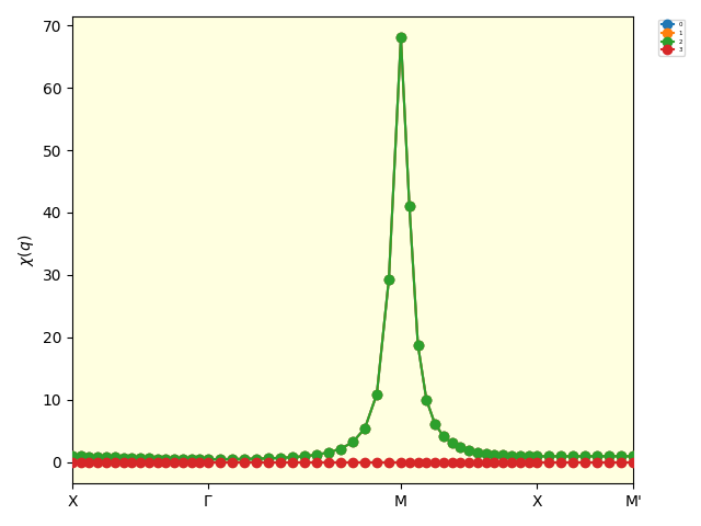
The eigenvalues of the two-body susceptibility calculated by the SCL.