Multiple band Hubbard model
In this tutorial, we will calculate the susceptibility of the multiple band Hubbard model.
For details, see the section VII of the reference paper, J. Otsuki, et al., Phys. Rev. B 99, 165134 (2019).
Sample files for this tutorial are available at examples/two_orbital.
Model
where \(i\) is the site index and \(\alpha\), \(\beta\) are the orbital indices. \(\sigma\) is the spin index and \(\bar{\sigma}\) means the opposite spin of \(\sigma\). \(\varepsilon_{\boldsymbol{k}} = -2t(\cos k_x + \cos k_y)\) is the dispersion relation, \(\Delta_\alpha\) is the crystal field splitting, \(U\) is the intra-orbital Coulomb interaction, \(U'\) is the inter-orbital Coulomb interaction, and \(J\) is the Hund’s coupling. In this tutorial, we consider the two-band Hubbard model with the following parameters: \(t = 1\) (set as the unit of energy), \(U = 12.0\), \(U' = 6.0\), \(J = 3.0\), \(\Delta_0 = 8.8\), and \(\Delta_1 = -8.8\).
DMFT calculation with DCore
To implement this setup in DCore, we need to prepare the input file as follows:
[model]
seedname = square_2orb
lattice = wannier90
norb = 2
nelec = 2.0
t = -1.0
kanamori = [(12.0, 6.0, 3.0)]
nk0 = 32
nk1 = 32
nk2 = 1
local_potential_matrix = {0: 'local_pot.in'}
local_potential_factor = 8.8

#[mpi]
#command = "mpirun -n #"

[system]
T = 0.5
n_iw = 1024
# fix mu at half-filling
mu = 10.5
fix_mu = True

[impurity_solver]
name = pomerol
exec_path{str} = pomerol2dcore
n_bath{int} = 0
fit_gtol{float} = 1e-6

[control]
# No iteration is necessary because of fix_mu=True and n_bath=0
max_step = 1
sigma_mix = 1.0
converge_tol = 1e-5
n_converge = 3

[bse]
num_wb = 1
num_wf = 20
X0q_qpoints_saved = "q_path.dat"
As for the previous example for the single-band Hubbard model, the [model] section specifies the model parameters.
norb is set to 2 to specify the number of orbitals. nelec = 2 means that the number of electrons per site is 2 (half-filling).
The hopping constants are specified by the Wannier90 format file square_2orb_hr.dat.
When norb increases, the number of lines in this file will increase as \(O(n_{\text{orb}}^2)\).
Hence, a python script make_hr_norb.py is offered to generate this file as follows:
python3 make_hr_norb.py 2 > square_2orb_hr.dat
The kanamori section specifies the Kanamori interaction parameters \((U, U', J) = (12.0, 6.0, 3.0)\).
local_potential_matrix and local_potential_factor are used to specify the local_potential parameters.
In this case, local_potential_matrix points to the file containing the local potential matrix as follows:
# spin orb1 orb2  Re Im
0 0 0   0.5 0.
0 1 1  -0.5 0.
1 0 0   0.5 0.
1 1 1  -0.5 0.
and local_potential_factor is set to 8.8.
Once the input file is prepared, we can run the DMFT calculation as the previous example:
dcore_pre dmft_2orb.in
dcore --np 4 dmft_2orb.in
dcore_check dmft_2orb.in
BSE calculation
First, we need to generate the q-path file from the input file
# qx qy qz name  (in unit of reciprocal lattice vectors)
1/2 0 0  X
0 0 0  Gamma
1/2 1/2 0  M
1/2 0 0  X
1/4 1/4 0  M'
as follows:
gen_qpath.py dmft_2orb.in qpath.in
Next, we need to prepare the input file for the BSE calculation.
[chiq_common]
input = "dmft_bse.h5"
output = "dmft_bse.out.h5"
type = ["chi0", "bse"]  # "chi0", "bse", "scl", "rpa", "rrpa"
omega_q = "q_path.dat"

[chiq_main]
work_dir = "work/chiq"
# num_wf = 20  # If not specified, the value is determined from X_loc

[chiq_post]
output_dir = "bse"
mode = ["eigen"]  # "matrix_element", "eigen", "linear_combination"

# for mode="eigen"
#vector = true  # output eigenvectors
order = "file"  # "descend" (default), "overlap", "file"
order_file = "eigenvec.in"  # for order="file"

# for mode="linear_combination"
# coefs_file = "/path/to/coefs.in"
The [chiq_common] and [chiq_main] sections are the same as the previous example.
BSE calculation can be performed using the following commands:
dcore_chiq.py --np 4 bse.in
mpiexec --np 4 chiq_main.py bse.in
The obtained susceptibility is a 16x16 complex-valued matrix.
In this example, we transform the susceptibility to the basis described in the reference paper.
The transformation matrix is given by eigenvec.in as follows:
# from Table I in J. Otsuki et al. PRB 99, 165134 (2019)
# sigma^0  tau^0 : charge
0.5 0  0 0  0 0  0.5 0   0 0  0 0  0 0  0 0   0 0  0 0  0 0  0 0   0.5 0  0 0  0 0  0.5 0
#
# sigma^z  tau^0 : spin^z
0.5 0  0 0  0 0  0.5 0   0 0  0 0  0 0  0 0   0 0  0 0  0 0  0 0   -0.5 0  0 0  0 0  -0.5 0
# sigma^+  tau^0 : spin^+
0 0  0 0  0 0  0 0   0.707106781186 0  0 0  0 0  0.707106781186 0   0 0  0 0  0 0  0 0   0 0  0 0  0 0  0 0
# sigma^-  tau^0 : spin^-
0 0  0 0  0 0  0 0   0 0  0 0  0 0  0 0   0.707106781186 0  0 0  0 0  0.707106781186 0   0 0  0 0  0 0  0 0
#
# sigma^0  tau^z : orbital (Eg in Oh)
0.5 0  0 0  0 0  -0.5 0   0 0  0 0  0 0  0 0   0 0  0 0  0 0  0 0   0.5 0  0 0  0 0  -0.5 0
#
# sigma^0  tau^x : orbital (Eg in Oh)
0 0  0.5 0  0.5 0  0 0  0 0  0 0  0 0  0 0   0 0  0 0  0 0  0 0   0 0  0.5 0  0.5 0  0 0
#
# sigma^z  tau^y : orbital (T2g in Oh)
0 0  0.5 0  -0.5 0  0 0   0 0  0 0  0 0  0 0   0 0  0 0  0 0  0 0   0 0  -0.5 0  0.5 0  0 0
# sigma^+  tau^y : orbital (T2g in Oh)
0 0  0 0  0 0  0 0   0 0  0.707106781186 0  -0.707106781186 0  0 0   0 0  0 0  0 0  0 0   0 0  0 0  0 0  0 0
# sigma^-  tau^y : orbital (T2g in Oh)
0 0  0 0  0 0  0 0   0 0  0 0  0 0  0 0   0 0  0.707106781186 0  -0.707106781186 0  0 0   0 0  0 0  0 0  0 0
#
# sigma^0  tau^y : magnetic high-rank multipole (A1u in Oh)
0 0  0.5 0  -0.5 0  0 0   0 0  0 0  0 0  0 0   0 0  0 0  0 0  0 0   0 0  0.5 0  -0.5 0  0 0
#
# sigma^z  tau^x : magnetic high-rank multipole (T1u in Oh)
0 0  0.5 0  0.5 0  0 0  0 0  0 0  0 0  0 0   0 0  0 0  0 0  0 0   0 0  -0.5 0  -0.5 0  0 0
# sigma^+  tau^x : magnetic high-rank multipole (T1u in Oh)
0 0  0 0  0 0  0 0   0 0  0.707106781186 0  0.707106781186 0  0 0   0 0  0 0  0 0  0 0   0 0  0 0  0 0  0 0
# sigma^-  tau^x : magnetic high-rank multipole (T1u in Oh)
0 0  0 0  0 0  0 0   0 0  0 0  0 0  0 0   0 0  0.707106781186 0  0.707106781186 0  0 0   0 0  0 0  0 0  0 0
#
# sigma^z  tau^z : magnetic high-rank multipole (T2u in Oh)
0.5 0  0 0  0 0  -0.5 0   0 0  0 0  0 0  0 0   0 0  0 0  0 0  0 0   -0.5 0   0 0  0 0  0.5 0
# sigma^+  tau^z : magnetic high-rank multipole (T2u in Oh)
0 0  0 0  0 0  0 0   0.707106781186 0  0 0  0 0  -0.707106781186 0   0 0  0 0  0 0  0 0   0 0  0 0  0 0  0 0
# sigma^-  tau^z : magnetic high-rank multipole (T2u in Oh)
0 0  0 0  0 0  0 0   0 0  0 0  0 0  0 0   0.707106781186 0  0 0  0 0  -0.707106781186 0   0 0  0 0  0 0  0 0
This has the same format as the eigenvector file outputted by chiq_post.py.
To check these basis, use eigenvec_viewer.py as follows:
eigenvec_viewer.py eigenvec.in -a 1 --spin-charge
For example, the 11th eigenvector (#10) is as follows:
#10
atom 0
ch
  0               0
  0               0
sp+
  0               0
  0               0
sp-
  0               0
  0               0
spz
  0               0.707
  0.707           0
ch, sp+, sp-, and spz are the charge \(n\), spin-up \(\sigma^+\), spin-down \(\sigma^-\), and spin-z \(\sigma^z\), respectively.
\(2 \times 2\) matrices are the orbital components \(\tau\) coupled to each spin-charge component.
Therefore, this says that the 11th eigenvector is \(\sigma^z \times \tau^x\) (one of the \(T_{1u}\)).
Basis transformation is performed by chiq_post.py as follows:
chiq_post.py bse.in
The transformed susceptibility is stored in bse/chi_q_eigen.dat.
In the plotting tool, plot_chiq_path.py, you can select the susceptibility to plot by specifying the eigenvector index by using the following file, label.in:
# from Table I in J. Otsuki et al. PRB 99, 165134 (2019)
{
#		0: "charge",
		1: "spin",
		4: "HS/LS",
#		5: "tau^x",
		6: "orb^3",
#		9: "sp-orb^1",
		10: "EI",
#		13: "sp-orb^{3z}",
}
This file has a python dictionary, where the key is the eigenvector index and the value is the label in the plot.
Note that the line starting with # is a comment, and then the four bands, 1, 4, 6, and 10, are specified in this case.
label.in is passed to plot_chiq_path.py as follows:
plot_chiq_path.py q_path.dat bse/chi_q_eigen.dat --label=label.in
The obtained figure shows the susceptibility along the path in the Brillouin zone as follows:
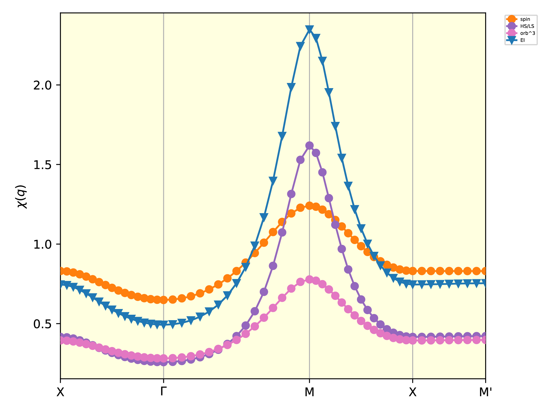
The susceptibility \(\chi(\boldsymbol{q})\) calculated by the BSE.