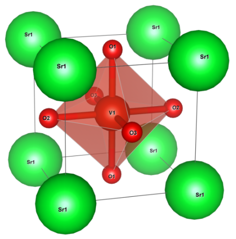
SrVO3
Note
This tutorial requires parallel computing.
Crystal structure of SrVO3 (drawn by VESTA).
Construction of Wannier functions
Maximally localized Wannier functions for the t2g manifold can be constructed by using DFT code. Please download precomputed data for Wannier functions
and save it to your working directly. This data was computed by using Quantum ESPRESSO and Wannier90. The procedure of Wanniernization is detailed in Wanniernization using Quantum ESPRESSO and Wanniernization using OpenMX.
DMFT calculation
[model]
lattice = wannier90
seedname = srvo3
nelec = 1.0
ncor = 1
norb = 3
kanamori = [(3.419, 2.315, 0.530)]
bvec=[(1.627091,0.0,0.0),(0.0,1.627091,0.0),(0.0,0.0,1.627091)]
nk0 = 10
nk1 = 10
nk2 = 10

#[mpi]
#command = '$MPIRUN -np #'

[system]
beta = 40.0
mu = 12.290722
with_dc = True

[impurity_solver]
name = ALPS/cthyb
timelimit{int} = 90
exec_path{str} = hybmat

[control]
max_step = 12
time_reversal = True
sigma_mix = 0.8

[post.spectrum]
broadening = 0.1
nk_line = 50
knode=[(G,0.0,0.0,0.0),(X,0.5,0.0,0.0),(M,0.5,0.5,0.0),(G,0.0,0.0,0.0),(R,0.5,0.5,0.5)]

[post.anacont]
omega_max =2.0
omega_min =-2.0
Nomega = 400

[post.anacont.pade]
iomega_max = 2.0

[post.check]
omega_check = 30.0
To use TRIQS/cthyb, please use
[model]
lattice = wannier90
seedname = srvo3
nelec = 1.0
ncor = 1
norb = 3
kanamori = [(3.419, 2.315, 0.530)]
bvec=[(1.627091,0.0,0.0),(0.0,1.627091,0.0),(0.0,0.0,1.627091)]
nk0 = 10
nk1 = 10
nk2 = 10

#[mpi]
#command = '$MPIRUN -np #'

[system]
beta = 40.0
mu = 12.290722
with_dc = True

[impurity_solver]
name = TRIQS/cthyb
n_cycles{int} = 10000
n_warmup_cycles{int} = 10000
length_cycle{int} = 400
move_double{bool} = True

[control]
max_step = 12
time_reversal = True
sigma_mix = 0.8

[post.spectrum]
broadening = 0.1
nk_line = 50
knode=[(G,0.0,0.0,0.0),(X,0.5,0.0,0.0),(M,0.5,0.5,0.0),(G,0.0,0.0,0.0),(R,0.5,0.5,0.5)]

[post.anacont]
omega_max =2.0
omega_min =-2.0
Nomega = 400

[post.anacont.pade]
iomega_max = 2.0

[post.check]
omega_check = 30.0
instead. Please see CT-QMC: TRIQS/cthyb for the details of the parameter setting for TRIQS/cthyb.
To generate reference data, we used 48 MPI processes (ISSP system B). The total computational time for 12 iterations is around 30 mins.
The accuracy of QMC results can be improved by setting a longer simulation time (ALPS/CT-HYB) or a larger n_cycles (TRIQS/cthyb). For ALPS/CT-HYB, the parameter time_limit is given in seconds.
DMFT setup: dcore_pre
$ dcore_pre srvo3.ini
Running self-consistent DMFT calculation: dcore
$ dcore srvo3.ini --np 48
Post-processing and data analysis: dcore_anacont and dcore_spectrum
$ dcore_anacont srvo3.ini
$ dcore_spectrum srvo3.ini --np 48
$ cd post
$ gnuplot akw.gp
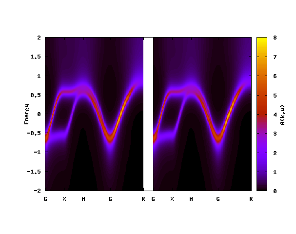
The left and right panels show results for up and down spins, respectively.