4.1. Ising model with transverse magnetic field

This section presents a calculation of the transverse magnetic field Ising model as an example. The Hamiltonian is

\[\begin{aligned} H = J^z \sum_{\langle i,j \rangle} {S}_i^{z} {S}_j^{z} - h^x \sum_i S_i^x. \end{aligned}\]

Please note that the model is defined using spin operators of size 1/2, not Pauli operators. By changing the variable hx in the input file, the magnitude of the transverse magnetic field will be modified. For example, when the transverse magnetic field is 0, the input file is

[parameter]
[parameter.general]
is_real = true  # Limit tensor elements in real (not complex)

[parameter.simple_update]
num_step = 1000 # Number of steps in simple update
tau = 0.01      # Imaginary time slice

[parameter.full_update]
num_step = 0    # Number of steps in full update
tau = 0.01      # Imaginary time slice

[parameter.ctm]
meanfield_env = false # Use meanfield environment to contract iTNS
iteration_max = 10    # Maximum number of iterations in CTMRG
dimension = 10        # Bond dimension of corner transfer matrix

[lattice]
type = "square lattice" # Type of lattice
L = 2                   # X length of unit cell
W = 2                   # Y length of unit cell
virtual_dim = 2         # Bond dimension of bulk tensors
initial = "ferro"       # Initial condition

[model]
type = "spin" # Type of model
Jz = -1.0     # Jz SzSz
Jx = 0.0      # Jx SxSx
Jy = 0.0      # Jy SySy
hx = 0.0      # hx Sx

In this case, since Jz = -1.0 , the ferromagnetic state manifests itself as the ground state at hx=0. When the input file name is simple.toml , type the following commands to execute tenes (before typing them, please install TeNeS and set PATH properly.):

$ tenes_simple simple.toml
$ tenes_std std.toml
$ tenes input.toml

Then, the following logs are output:

Number of Processes: 1
Number of Threads / Process: 1
Tensor type: real
Start simple update
10% [100/1000] done
20% [200/1000] done
30% [300/1000] done
40% [400/1000] done
50% [500/1000] done
60% [600/1000] done
70% [700/1000] done
80% [800/1000] done
90% [900/1000] done
100% [1000/1000] done
Start calculating observables
Start updating environment
Start calculating onesite operators
Save onesite observables to output_0/onesite_obs.dat
Start calculating twosite operators
Save twosite observables to output_0/twosite_obs.dat
Save observable densities to output_0/density.dat
Save elapsed times to output_0/time.dat

Onesite observables per site:
Sz          = 0.5 0
Sx          = -1.28526262482e-13 0
Twosite observables per site:
hamiltonian = -0.5 0
SzSz        = 0.5 0
SxSx        = -1.7374919982e-18 0
SySy        = 1.73749202733e-18 0
Wall times [sec.]:
simple update = 3.545813509
full update   = 0
environmnent  = 0.123170523
observable    = 0.048149856

Done.

First, the information of parallelization and the tensors (complex or not) is displayed. Next, the execution status of the calculation process is displayed. After finishing the calculation, the expected values per site of the one-site operators Sz, Sx and two-site ones Hamiltonian, the nearest correlation SzSz, SxSx, SySy are output. Finally, the calculation time for each process is output in units of seconds. density.dat, parameters.dat, time.dat, onesite_obs.dat, and twosite_obs.dat are saved to the output directory. For details on each output file, see Output files. For example, the value of <Sz> can be read from onesite_obs.dat. By changing hx in increments of 0.2 from 0 to 3.0 and running tenes_simple and tenes, the following result is obtained. As an example of the sample script, tutorial_example.py , tutorial_read.py are prepared in the sample/01_transverse_field_ising directory.

• tutorial_example.py

import subprocess

import numpy as np
import toml

MPI_cmd = ""  # e.g., "mpiexec -np 1"

num_hx = 16
min_hx = 0.0
max_hx = 3.0

total = 0
for idx, hx in enumerate(np.linspace(min_hx, max_hx, num=num_hx)):
    print(f"Calculation Process: {idx+1}/{num_hx}")
    with open("simple.toml") as f:
        dict_toml = toml.load(f)
    dict_toml["parameter"]["general"]["output"] = f"output_{idx}"
    dict_toml["model"]["hx"] = float(hx)

    simple_toml = f"simple_{idx}.toml"
    std_toml = f"std_{idx}.toml"
    input_toml = f"input_{idx}.toml"

    with open(simple_toml, "w") as f:
        toml.dump(dict_toml, f)
    cmd = f"tenes_simple {simple_toml} -o {std_toml}"
    subprocess.call(cmd.split())

    cmd = f"tenes_std {std_toml} -o {input_toml}"
    subprocess.call(cmd.split())

    cmd = f"{MPI_cmd} tenes {input_toml}"
    subprocess.call(cmd.split())

• tutorial_read.py

from os.path import join

import toml

num_hx = 16

print("# $1: h")
print("# $2: ene")
print("# $3: sz")
print("# $4: sx")
print()

for idx in range(num_hx):
    try:
        with open(f"simple_{idx}.toml") as f:
            dict_toml = toml.load(f)
        hx = dict_toml["model"]["hx"]
        ene = 0.0
        mag_sz = 0.0
        mag_sx = 0.0
        with open(join(f"output_{idx}", "density.dat")) as f:
            for line in f:
                words = line.split()
                if words[0] == "Energy":
                    ene = words[2]
                elif words[0] == "Sz":
                    mag_sz = words[2]
                elif words[0] == "Sx":
                    mag_sx = words[2]
        print(f"{hx} {ene} {mag_sz} {mag_sx}")
    except:
        continue

The calculation will be done by typing the following command:

$ python tutorial_example.py

For MacBook2017 (1.4 GHz Intel Core i7), the calculation was finished in a few minutes. By typing the following command, hx, energy, <Sz> and <Sx> are outputted in the standard output:

$ python tutorial_read.py

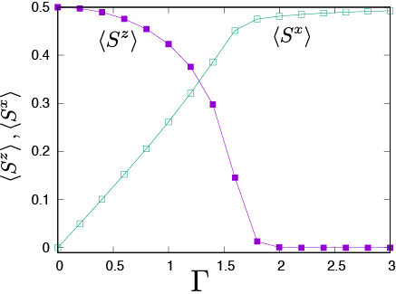
Fig. 4.1 hx dependence of <Sz> and <Sx>.

As seen from Fig. 4.1 , with increasing hx, the <Sz> decreases from 0.5 to 0, while the <Sx> increases from 0 to 0.5.