4.6. Definition of lattices, models, and operators using the standard mode

By using the standard mode, users can define own lattices, models, and operators. In this section, we explain how to use the standard mode.

4.6.1. Definition of unit cell

Fig. 4.8 [tensor] and [[tensor.unitcell]]

Unit cells are defined using [tensor] and [[tensor.unitcell]]:

[tensor]
L_sub = [2, 2]          # 2x2 unitcell
skew = 0                # Displacement in x direction
                        # when go beyond a y-direction boundary

[[tensor.unitcell]]
virtual_dim = [4, 4, 4, 4] # Bond dimensions (←, ↑, →, ↓)
index = [0, 3]             # Indices of tensors in the unit cell
physical_dim = 2           # Physical bond dimensions
initial_state = [1.0, 0.0] # Initial state coefficients
noise = 0.01               # Fluctuation of elements in initial tensor

The initial state \(\ket{\Psi}\) is prepared as the direct product state of the per-site initial states \(\ket{\psi}_i\) : \(\ket{\psi} = \otimes_i \ket{\psi_i}\). \(\ket{\psi}_i\) can be specified as follows, with the elements of the initial_state = [a0, a1, ..., a_{d-1}],

\[\Ket{\psi}_i \propto \sum_{k=0}^{d-1}a_k\Ket{k}\]

4.6.2. Definition of model (Hamiltonian)

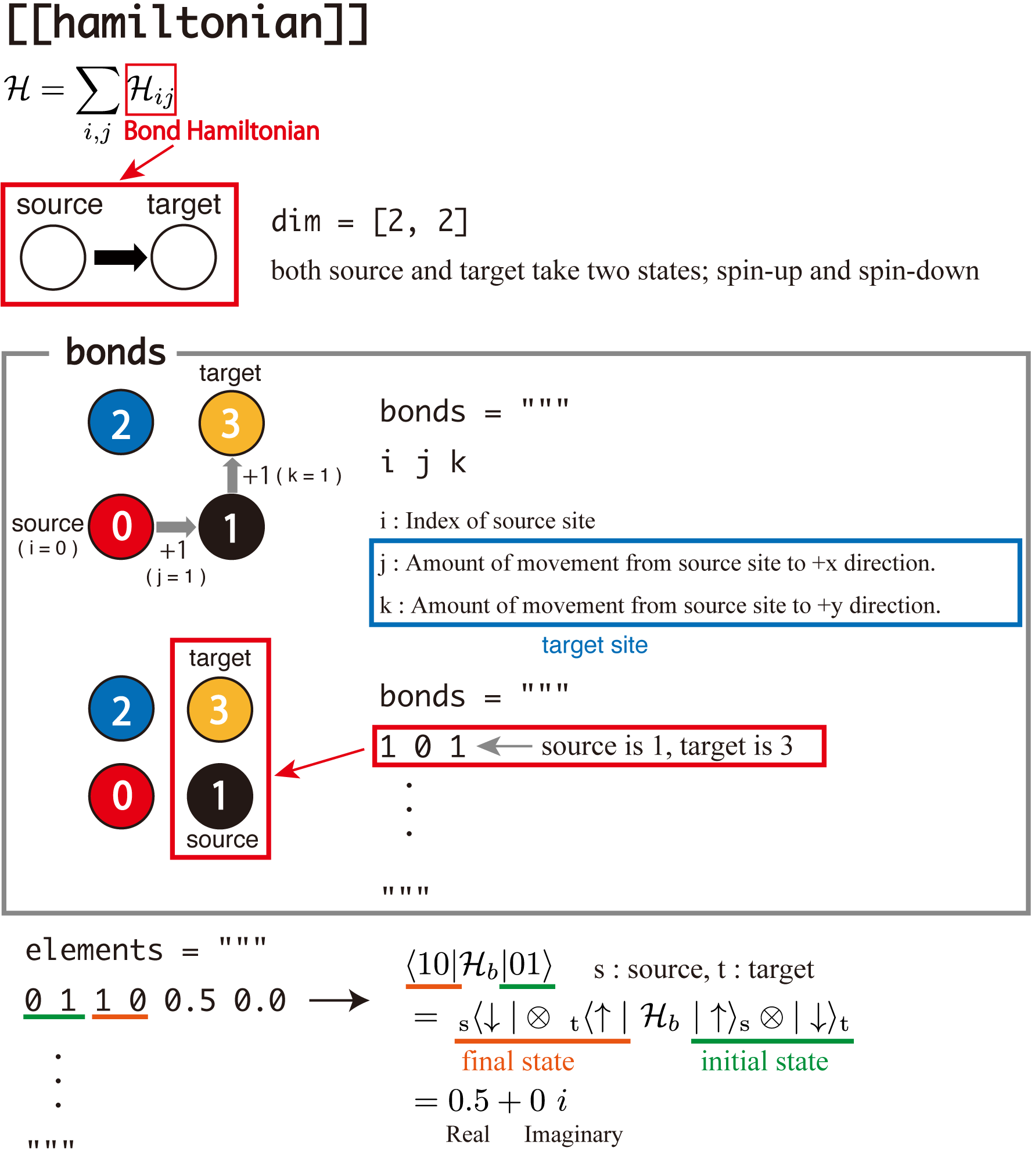
Fig. 4.9 [[hamiltonian]]

TeNeS treats the Hamiltonian as the sum of bond Hamiltonians (two-site Hamiltonians) and site Hamiltonians (one-site Hamiltonians).

\[mathcal{H} = \sum_{i,j}\mathcal{H}_{i,j} + \sum_{i} \mathcal{H}_i\]

These local Hamiltonians are defined as pairs of (nonzero) elements of matrix and site/bond it acts on. A bond is a directed pair of two sites: source and target. To define matrix elements is to define a model, and to define bonds is to define a lattice.

Bond Hamiltonian

In the input file of the standard mode, say std.toml, each local Hamiltonian is specified as [[hamiltonian]]. The bonds where the bond Hamiltonian acts are specified by bonds string:

[[hamiltonian]]
bonds = """ # Set of acting bonds (1 bond per line)
0 1 0       # Row 1: Number of the source in the unit cell
1 1 0       # Row 2: x coordinate(displacement) of target from the source
2 1 0       # Row 3: y coordinate(displacement) of target from the source
3 1 0
0 0 1
1 0 1
2 0 1
3 0 1
"""

One line of three integers corresponds one bond. The first integer is the index of the source site. The other two integers are x and y displacement of the target site from the source site. For example, 0 1 0 means the pair of the site 0 and the right neighbor (x+=1 and y+=0), the site 1, and 1 0 1 means the pair of the site 1 and the top neighbor (x+=0 and y+=1), the site 3.

The dimension of the bond Hamiltonian, i.e., the number of states of the source and target sites, is specified by dim, and the non-zero elements of the bond Hamiltonian is defined by elements:

dim = [2, 2]       # Number of possible states of the acting bond [source, target]
elements = """     # (nonzero) matrix elements of the Hamiltonian (one element per row)
0 0 0 0 0.25 0.0   # Field 1: State of source before action
1 0 1 0 -0.25 0.0  # Field 2: State of target before action
0 1 1 0 0.5 0.0    # Field 3: State of source after action
1 0 0 1 0.5 0.0    # Field 4: State of target after action
0 1 0 1 -0.25 0.0  # Field 5: Real part of element
1 1 1 1 0.25 0.0   # Field 6: Imaginary part of element
"""

One line of elements corresponds one element. The first two integers are the states of the source and target sites before the Hamiltonian acts on, and the following two integers are the states of the source and target sites after the Hamiltonian acts on. The remaining two numbers are the real and imaginary part of the element of the bond Hamiltonian.

Site Hamiltonian

A site Hamiltonian is defined as a pair of (non-zero) matrix element and site it acts on.:

[[hamiltonian]]
dim = [2]
sites = []
elements = """
1 0 -0.5 0.0
0 1 -0.5 0.0
"""

Site is specified by sites as a list of indices. An empty list means all the sites.

Non-zero matrix elements are specified by elements, and how to define is the similar for bond Hamiltonians (Note that site Hamiltonians acts on only one site).

4.6.3. Definition of operators

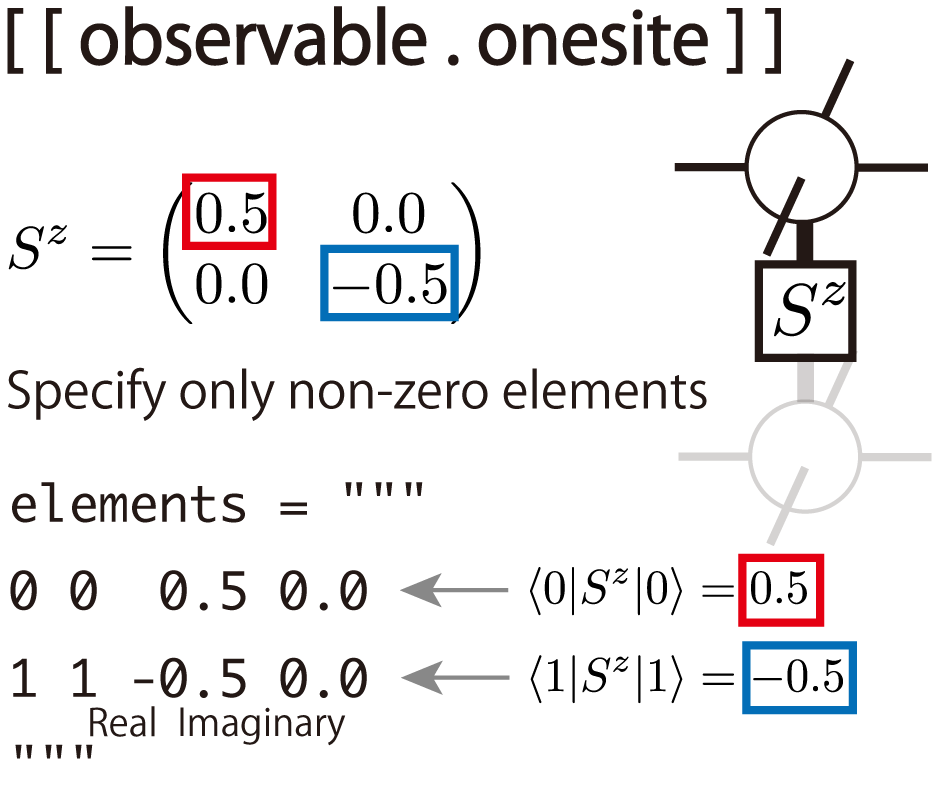
Fig. 4.10 [[observable.onesite]]

Operators whose expected values are finally computed are defined in [observable]. The current version of TeNeS can evaluate onesite and twosites operators. The way to define operators is similar in Hamiltoninans, but an operator require the name (name) and identifier number (group). Although the energy operator is just the Hamiltonian (sum of the bond Hamiltonians), it should be defined in [observable] if users want to calculate. For convenience, tenes_std copies [[hamiltonian]] in [[observable]] when operator with group = 0 is not defined.

For an example of onesite operator, the z-component of the spin operator

S^z = \begin{pmatrix}
0.5 & 0.0 \\
0.0 & -0.5 \\
\end{pmatrix}

is defined as follows:

[[observable.onesite]] # onesite operator
name = "Sz"            # Name
group = 0              # 1-site operator identification number
sites = []             # Indices of tensors on which the operator acts ([] means all)
dim = 2                # Dimensions of operators
elements = """         # Non-zero elements of operator matrix (one element per line)
0 0 0.5 0.0            # Fields 1 and 2: before and after action
1 1 -0.5 0.0           # Fields 3 and 4: Real and imaginary parts of the element
"""

Non-zero elements of the matrix can be specified in the similar way of bond Hamiltonians.

Twosites operators can be defined in the similar way how to define the bond Hamiltonian. As an example of twosites operator, spin-spin correlation on nearest neighbor bonds \(S^z_i S^z_j\) is defined as follows:

[[observable].twosite]] # twosite operator
name = "SzSz"           # Name
group = 1               # Index of twosite operator (independent of indices of onesite)
dim = [2, 2]            # Dimension
bonds = """             # Bond that acts on
0 1 0
1 1 0
2 1 0
3 1 0
0 0 1
1 0 1
2 0 1
3 0 1
"""
ops = [0, 0] # When it can be written as a direct product of onesite operators,
             # their indices.
             # In this case, "Sz" is the onesite operator with index 0.
             # Matrix elements can also be written explicitly as elements

When the twosites operator is written as the direct product of the two onesite operators, ops can be used to specify them.

4.6.4. Example: Antiferromagnetic Heisenberg model in staggered field

Let us consider the antiferromagnetic Heisenberg model in staggered field. The Hamiltonian is as follows

\[\mathcal{H} = J \sum_{\braket{ij}} S_i \cdot S_j - h \sum_{i \in A} S_i^z + h \sum_{j \in B} S_j^z,\]

where \(\sum_{\braket{ij}}\) is summation over the nearest neighbor bonds and \(A\) and \(B\) are the sublattices of the square lattice. The bond Hamiltonian \(\mathcal{H}_{ij}\) can be written as follows

\[\begin{split}\begin{split} \mathcal{H}_{ij} &= J S_i \cdot S_j \\ &= \begin{pmatrix} J/4 & 0 & 0 & 0 \\ 0 & -J/4 & J/2 & 0 \\ 0 & J/2 & -J/4 & 0 \\ 0 & 0 & 0 & J/4 \\ \end{pmatrix} \end{split}\end{split}\]

and the site Hamiltonian \(\mathcal{H}_i\) can be written as

\[\begin{split}\begin{split} \mathcal{H}_{i} &= -h S_i^z \\ &= \begin{pmatrix} -h/2 & 0 \\ 0 & h/2 \\ \end{pmatrix} \end{split}\end{split}\]

When \(J = 0, h = 1\), for example, an input file of tenes_std, std.toml (sample/06_std_model/std.toml), is as follows

[parameter]
[parameter.general]
is_real = true
tensor_save = "tensor"
[parameter.simple_update]
num_step = 1000
tau = 0.01
[parameter.full_update]
num_step = 0
tau = 0.01
[parameter.ctm]
iteration_max = 10
dimension = 10

[tensor]
type = "square lattice"
L_sub = [2, 2]
skew = 0

[[tensor.unitcell]]
virtual_dim = [2, 2, 2, 2]
index = [0, 3]
physical_dim = 2
initial_state = [1.0, 0.0]
noise = 0.01

[[tensor.unitcell]]
virtual_dim = [2, 2, 2, 2]
index = [1, 2]
physical_dim = 2
initial_state = [0.0, 1.0]
noise = 0.01

[[hamiltonian]]
dim = [2]
sites = [0, 3]
elements = """
0 0 -0.5 0.0
1 1 0.5 0.0
"""

[[hamiltonian]]
dim = [2]
sites = [1, 2]
elements = """
0 0 0.5 0.0
1 1 -0.5 0.0
"""

[observable]
[[observable.onesite]]
name = "Sz"
group = 1
sites = []
dim = 2
elements = """
0 0 0.5 0.0
1 1 -0.5 0.0
"""

[[observable.twosite]]
name = "SzSz"
group = 1
dim = [2, 2]
bonds = """
0 1 0
1 1 0
2 1 0
3 1 0
0 0 1
1 0 1
2 0 1
3 0 1
"""
ops = [1, 1]

We can calculate this model and obtain results as

$ tenes_std std.toml
$ tenes input.toml

   ... skipped ...

Onesite observables per site:
  hamiltonian = -0.5 0
  Sz          = 0 0
Twosite observables per site:
  SzSz        = -0.5 0

   ... skipped

Especially, the expectation values of onesite operators written in output/onesite_obs.dat are:

# $1: op_group
# $2: site_index
# $3: real
# $4: imag

0 0 -5.00000000000000000e-01 0.00000000000000000e+00
0 1 -5.00000000000000000e-01 0.00000000000000000e+00
0 2 -5.00000000000000000e-01 0.00000000000000000e+00
0 3 -5.00000000000000000e-01 0.00000000000000000e+00
1 0 5.00000000000000000e-01 0.00000000000000000e+00
1 1 -5.00000000000000000e-01 0.00000000000000000e+00
1 2 -5.00000000000000000e-01 0.00000000000000000e+00
1 3 5.00000000000000000e-01 0.00000000000000000e+00
-1 0 2.20256797875764860e+04 0.00000000000000000e+00
-1 1 2.20198975366861232e+04 0.00000000000000000e+00
-1 2 2.20294461413457539e+04 0.00000000000000000e+00
-1 3 2.20236290136460302e+04 0.00000000000000000e+00

Values of \(S^z\) (op_group=) show that spins on the A sublattice (site_index=0,3) are up (0.5) and those on the B (site_index=1,2) are down (-0.5). By imposing the staggered magnetic field (\(J = 0, h = 1\)), a tensor product state representing the Neel state is obtained. Tensors are saved into the tensor directory because we set tensor_save = "tensor", and therefore we can use them as the initial states of another calculation by setting tensor_load = "tensor".