4.4. Magnetization process of the Heisenberg model on triangular and square lattices

Next, we introduce the calculation of the magnetization process of the quantum Heisenberg model with spin \(S = 1/2\) defined on a triangular lattice. The Hamiltonian looks like this:

\[\begin{aligned} H = J \sum_{\langle i,j \rangle}\sum_{\alpha}^{x,y,z} {S}_i^{\alpha} {S}_j^{\alpha} - h \sum_i S_i^z\end{aligned}\]

Here, \(\langle i, j \rangle\) represents the pair of nearest neighbor sites, and \(h\) represents the magnitude of the external magnetic field applied in the \(z\) direction. Let’s calculate the ground state of this model and find \(\langle S_z \rangle\equiv \frac{1}{N_u}\sum_i^{N_u} \langle S_i^z \rangle\), where \(N_u\) is the total number of sites in the unit cell, as a function of the magnetic field \(h\). To do this, the toml file basic.toml and the python script tutorial_magnetization.py are prepared in the sample/04_magnetization directory. The basic.toml file contains model settings and parameters.

[parameter]
[parameter.general]
is_real = true

[parameter.simple_update]
num_step = 200
tau = 0.01

[parameter.full_update]
num_step = 0
tau = 0.01

[parameter.ctm]
iteration_max = 100
dimension = 10

[lattice]
type = "triangular lattice"
L = 3
W = 3
virtual_dim = 2
initial = "random"

[model]
type = "spin"
J = 1.0

The lattice section specifies a triangular lattice with the unit cell size of \(3\times 3\). Here, in order to make the calculation lighter, only simple update is performed, and the imaginary time interval \(\tau\) is assumed to be \(\tau = 0.01\). For simplicity, \(J=1\). Using this basic setting file, tutorial_magnetization.py calculates the magnetization when the magnetic field is swept.

import subprocess
from os.path import join
import numpy as np
import toml

MPI_cmd = ""  # e.g., "mpiexec -np 1"

num_h = 21
min_h = 0.0
max_h = 5.0
num_step_table = [100, 200, 500, 1000, 2000]

fmag = open("magnetization.dat", "w")
fene = open("energy.dat", "w")

for f in (fmag, fene):
    f.write("# $1: hz\n")
    for i, num_step in enumerate(num_step_table, 2):
        f.write(f"# ${i}: num_step={num_step}\n")
    f.write("\n")

for idx, h in enumerate(np.linspace(min_h, max_h, num=num_h)):
    print(f"Calculation Process: {idx+1}/{num_h}")
    inum = 0
    num_pre = 0
    fmag.write(f"{h} ")
    fene.write(f"{h} ")
    for num_step in num_step_table:
        ns = num_step - num_pre
        print(f"Steps: {num_step}")
        with open("basic.toml") as f:
            dict_toml = toml.load(f)

        output_dir = f"output_{idx}_{num_step}"

        dict_toml["parameter"]["general"]["output"] = output_dir
        dict_toml["parameter"]["general"]["tensor_save"] = "tensor_save"
        dict_toml["model"]["hz"] = float(h)
        dict_toml["parameter"]["simple_update"]["num_step"] = ns
        if inum > 0:
            dict_toml["parameter"]["general"]["tensor_load"] = "tensor_save"

        simple_toml = f"simple_{idx}_{num_step}.toml"
        std_toml = f"std_{idx}_{num_step}.toml"
        input_toml = f"input_{idx}_{num_step}.toml"

        with open(simple_toml, "w") as f:
            toml.dump(dict_toml, f)
        cmd = f"tenes_simple {simple_toml} -o {std_toml}"
        subprocess.call(cmd.split())

        cmd = f"tenes_std {std_toml} -o {input_toml}"
        subprocess.call(cmd.split())

        cmd = f"{MPI_cmd} tenes {input_toml}"
        subprocess.call(cmd.split())

        ene = 0.0
        mag_sz = 0.0
        with open(join(output_dir, "density.dat")) as f:
            for line in f:
                name, vals = line.split("=")
                if name.strip() == "Energy":
                    re, im = vals.split()
                    ene += float(re)
                elif name.strip() == "Sz":
                    re, im = vals.split()
                    mag_sz += float(re)
        fene.write(f"{ene} ")
        fmag.write(f"{mag_sz} ")
        inum = inum + 1
        num_pre = num_step
    fene.write("\n")
    fmag.write("\n")
fene.close()
fmag.close()

In this script, the magnetic field \(h\) is changed in steps of \(0.25\) from \(0\) to \(5\), and the ground state energy and \(\langle S_z \rangle\) are calculated and output to energy.dat and magnetization.dat, respectively. In order to see what happens when the number of time steps for simple update is changed, calculations are also performed with \(100\), \(200\), \(500\), \(1000\), and \(2000\) steps for each magnetic field. In order to reduce the amount of calculation, the information of the wave function obtained with a small number of steps is stored in tensor_save, and this is used as the initial state for the calculation of a larger number of steps. For example, the python script first performs a calculation with the number of time steps set to 100, and output the result. Then, it perform a calculation with the number of time steps set to 200 using the wave function at the end of the calculation of the number of steps 100. The script consequently reduce the amount of the calculation by 100 steps for the latter in the directory.

Let’s actually run it. After passing through a path to tenes in advance, execute calculation by typing as follows.

python tutorial_magnetization.py

The calculation will finish within a few hours if you use a notebook PC using a single processor. After the calculation is completed, start up gnuplot and type

load 'plot.gp'

to obtain the magnetization curve as shown in the right panel of Fig. 4.5. In a similar way,

load 'plot_ene.gp'

we obtain the ground-state energy as shown in the left panel of Fig. 4.5 .

As can be seen from the result for a sufficiently large number of steps (for example, 2000 steps), a plateau structure occurs in the magnetization process at the magnetization of \(1/3\) of the saturation magnetization \(\langle S_z \rangle = 0.5\). On this plateau, spins on the three lattices form a periodic magnetic structure with \(\uparrow\), \(\uparrow\), \(\downarrow\), and a spin gap is generated. This plateau structure is unique to the triangular lattice. To see whether the accuracy of calculation is enough or not, it is helpful to check the step dependence of energy. In principle, the ground-state energy should decrease as the number of steps increases, but in some magnetic fields, the calculated energy increases. This is a sign that the calculation accuracy is not good. It is presumed that it is necessary to increase the bond dimension.

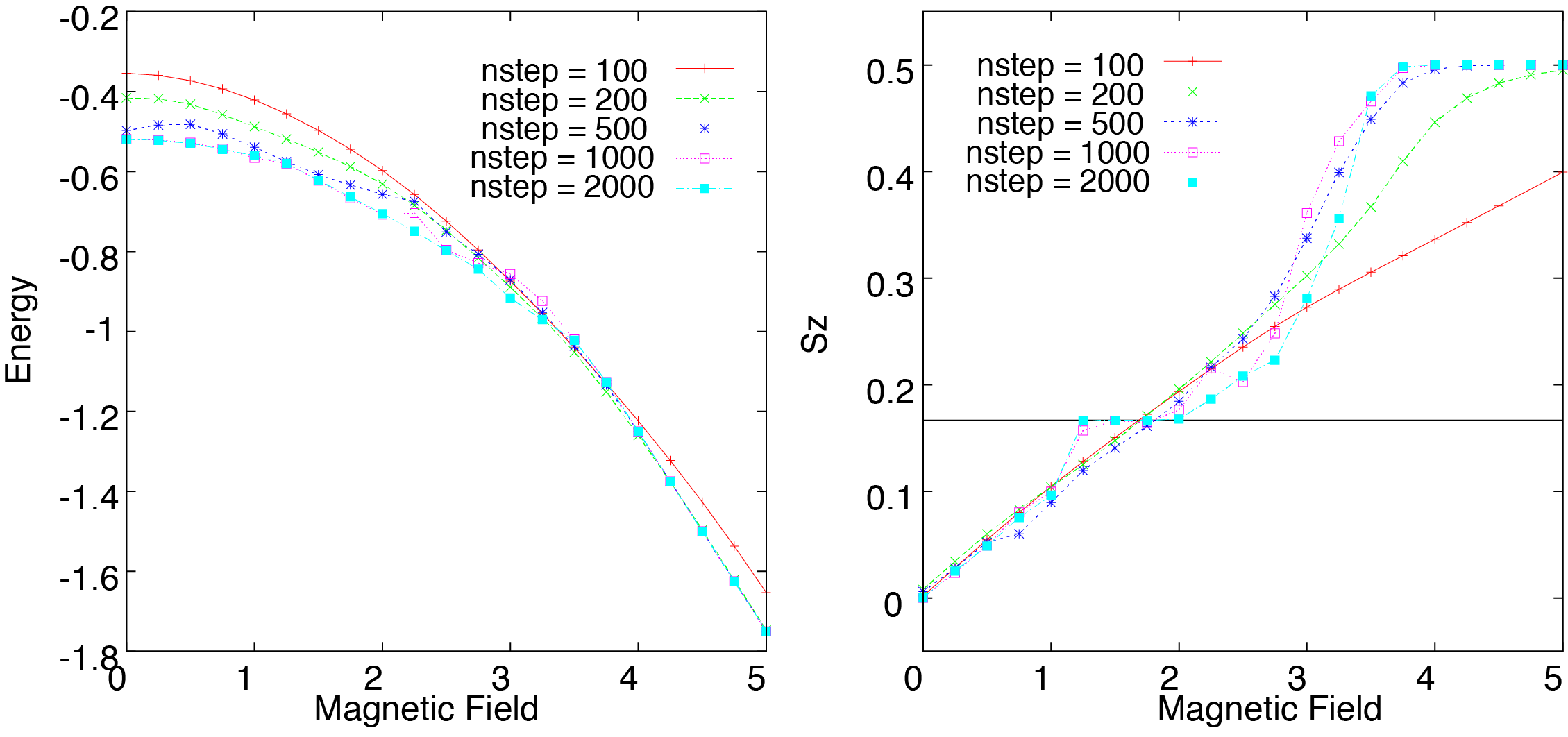
Fig. 4.5 Ground state energy (left figure) and magnetization (right figure) of the Heisenberg model on the triangular lattice.

Next, let’s perform the calculation for a model on a square lattice. Use the toml file basic_square.toml and the python script tutorial_magnetization_square.py in the sample/04_magnetization directory. The content of basic_square.toml is the same as basic.toml except that the lattice section has been changed as follows.

[lattice]
type = "square lattice"
L = 2
W = 2

To perform the calculation, type:

python tutorial_magnetization_square.py

After the calculation is completed, start up gnuplot and type

load 'plot_square.gp'

Then, the magnetization curve shown in the right panel of Fig. 4.6 is obtained. In a similar way, by typing the following command,

load 'plot_square_ene.gp'

you will obtain the ground-state energy as shown in the left panel of Fig. 4.6. The calculation is almost converged at 2000 steps, and it can be seen that the plateau structure does not appear unlike the triangular lattice Heisenberg model. Since the energy generally decreases as the number of steps is increased, it is assumed that the calculation accuracy is sufficiently high.

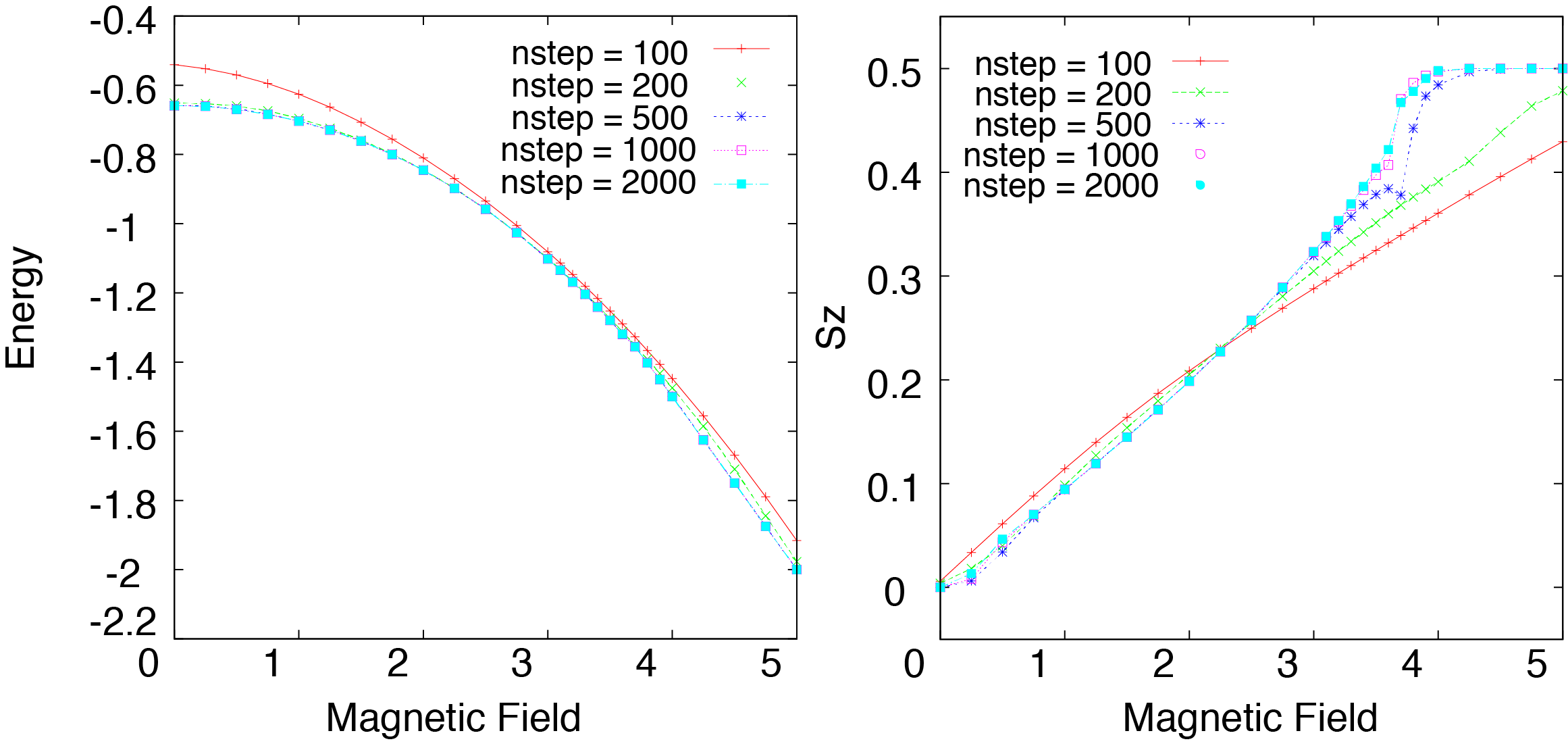
Fig. 4.6 Ground state energy (left figure) and magnetization (right figure) of the Heisenberg model on the square lattice.