4.1. Constructing a neural network model

This section contains instructions on how to construct a neural network using aenet to reproduce first-principles energies from Quantum ESPRESSO (QE). Here, we will consider the temperature-dependent degree of Mg/Al inversion in MgAl2O4 spinel. In the ground state, all Mg ions are tetrahedrally coordinated by O ions while Al ions are octahedrally coordinated. We will simulate the amount of inversion between these sites vs. temperature. The set of input files used in this tutorial can be found in examples/active_learning_qe. In the following, we briefly describe the installation of aenet and GNU parallel, but you may skip the section if they are preinstalled in your system. We will also use ohtaka, the supercomputer system B of the Institute for Solid State Physics, as the environment for running the calculations.

4.1.1. Preparation

Installation of aenet

In abICS, we use aenet to build neural network models. You can download aenet from http://ann.atomistic.net. Follow the Installation instructions in the Documentation to install it. Note that abICS uses generate.x, train.x and predict.x of aenet for training and evaluating neural networks. For train.x, an MPI parallel version can be used, but for generate.x and predict.x, you need to use a non-MPI executable file (serial). For this reason, you should also install the serial version under makefiles.

Installation of GNU parallel

In this tutorial, we will use GNU parallel to run first-principles calculations with Quantum Espresso in parallel. Therefore, you need to install GNU parallel first. GNU parallel can be downloaded from https://www.gnu.org/software/parallel/ (on a Mac, it can also be installed directly by homebrew). After moving to the directory where you downloaded and extracted the source files, you can install it into $HOME/opt/parallel by typing the following command.

$ ./configure --prefix=$HOME/opt/parallel
$ make && make install

For detailed configuration, please refer to the official manual.

4.1.2. Preparation of input files for training data set generation

A set of training data is required for creating a neural network that relate the configurations of atoms as input and the energy as output by the first-principle calculations. To generate the data set, the input files need to be prepared for both abICS and the first-principle solver.

Preparation of the abICS control file (input.toml)

This file contains the definition of the lattice structure to be calculated, the control of the entire active learning cycles by abICS, and the parameters for the replica exchange Monte Carlo method. By using the st2abics tool, you can automatically generate the input.toml template from the crystal structure file.

$ cd [example_dir].
$ st2abics st2abics_MgAl2O4.toml MgAl2O4.vasp > input.toml

In this section, we will explain the settings for each section of input.toml in more detail.

(i) [mlref] section

[mlref]
nreplicas = 8
ndata = 5

In this section, you can set the options for extracting atomic configurations from the RXMC calculation results to evaluate the accuracy of the neural network model and to expand the training data. Basically, nreplicas should be the same values as in the [sampling] section. ndata specifies how many samples to be extracted as the training dataset of the machine learning model from configurations generated by the RXMC calculation. Therefore, it should be set to a value less than or equal to the number of configurations generated by the RXMC calculation, nsteps/sample_frequency in [sampling] section.

(ii) [mlref.solver] section

[mlref.solver] # Set up a reference ab initio solver.
type = 'qe'
base_input_dir = ['./baseinput_ref', './baseinput_ref', './baseinput_ref'] #, './baseinput_ref']
perturb = 0.05

Set up the solver used to calculate the energy for training data (configuration energy). In this example, Quantum Espresso is used. The base_input_dir can be set freely. The input files for the solver are placed in the set directory (see below). If multiple directories are set up in a list format, as in this example, calculations using each input are performed in turn. The second and subsequent calculations will use the structure from the last step of the previous calculation as the initial coordinates. The energy of the last calculation is then used for training of the neural network model. For example, one could perform a fast structural optimization in the first input file at the expense of accuracy, and then perform a structural optimization in the second and subsequent input files with a higher accuracy setting. For another example, in the case of a lattice vector relaxation, the same input can be run multiple times to reset the computational mesh based on a set plane-wave cutoff.

The perturb is for starting the structural optimization from a structure with broken symmetry by randomly displacing each atom. In this case, the first calculation starts from the structure in which all atoms for structural relaxation are displaced by 0.05 angstrom in a random direction.

The ignore-species is set to an empty list when the first-principle solver is used for generating the training data. When a model is employed for the data generation in which some atomic species are ignored, they are specified in ignore-species.

(iii) [config] section

[config] # Set up information about the crystal lattice and the atoms and vacancies on the lattice.
unitcell = [[8.1135997772, 0.0000000000000000, 0.0000000000000000],
            [0.0000000000000000, 8.1135997772, 0.0000000000000000],
            [0.0000000000000000, 0.0000000000000000, 8.1135997772]]
supercell = [1,1,1]

[[config.base_structure]]
type = "O"
coords = [
    [0.237399980, 0.237399980, 0.237399980],
    [0.762599945, 0.762599945, 0.762599945],
    [0.512599945, 0.012600004, 0.737399936],
    [0.487399966, 0.987399936, 0.262599975],
    ...

[config] section specifies atomic positions to be used in the Monte Carlo sampling. The st2abics utility tool can generate this section. If abics_sampling has not been performed yet, the atomic positions are randomly generated based on this information, and the input files for the first-principle calculation are produced. Once abics_sampling is executed, the input files will be generated from the atomic positions obtained from the Monte Carlo sampling.

Preparation of the QE reference file

Place the input file to be referenced in the QE scf calculation in baseinput_ref. The following is a description of the scf.in file in the sample directory.

&CONTROL
calculation = 'relax'
tstress = .false.
tprnfor = .false.
pseudo_dir = './pseudo'
disk_io = 'low'
wf_collect = .false.
/
&SYSTEM
  ecutwfc = 60.0
  occupations = "smearing".
  smearing = "gauss"
  degauss = 0.01
/
&electrons
  mixing_beta = 0.7
  conv_thr = 1.0d-8
  electron_maxstep = 100
/
&ions
/
ATOMIC_SPECIES
Al 26.981 Al.pbe-nl-kjpaw_psl.1.0.0.UPF
Mg 24.305 Mg.pbe-spnl-kjpaw_psl.1.0.0.UPF
O 16.000 O.pbe-n-kjpaw_psl.1.0.0.UPF
ATOMIC_POSITIONS crystal

K_POINTS gamma

You need to rewrite the directory that contains the pseudopotentials, pseudo_dir, and the pseudopotentials used in ATOMIC_SPECIES according to your environment. The pseudopotentials used in this sample can be downloaded from the following link.

• https://pseudopotentials.quantum-espresso.org/upf_files/Al.pbe-nl-kjpaw_psl.1.0.0.UPF

• https://pseudopotentials.quantum-espresso.org/upf_files/Mg.pbe-spnl-kjpaw_psl.1.0.0.UPF

• https://pseudopotentials.quantum-espresso.org/upf_files/O.pbe-n-kjpaw_psl.1.0.0.UPF

In this example, calculation = 'relax' is used for structural optimization during the QE calculation, and gammma is used for K_POINTS to speed up the calculation.

4.1.3. Preparation of input files for training the neural network

In this tutorial we use aenet to train the neural netowrk. We need to prepare the input files for abICS and aenet.

Preparation of the abICS control file (input.toml)

(i) [train] section

[train] # Configure the model trainer.
type = 'aenet'
base_input_dir = '. /aenet_train_input'
exe_command = ['generate.x-2.0.4-ifort_serial',
              'srun train.x-2.0.4-ifort_intelmpi']
ignore_species = ["O"]

Set up a trainer to train a configuration energy prediction model from training data. Currently, abICS supports only aenet. You can freely set the base_input_dir. In that directory, set up the configuration files for the trainer (see below). In exe_command, specify the paths to generate.x and train.x of aenet. For train.x, an MPI parallel version is available, in which case, set the commands for MPI execution (mpiexec, srun, etc.) as shown in the example above.

The ignore-species is set to an empty list when the first-principle solver is used for generating the training data. When a model is employed for the data generation in which some atomic species are ignored, they are specified in ignore-species.

Preparation of input files for aenet

Place the input files for aenet in the generate, train, and predict directories in the directory set in the base_input_dir of the [train] section.

generate

aenet compiles the atomic configuration and energy data for training into an intermediate binary format that is converted into atomic environment descriptor-energy relationships before training. Input files for generate.x that perform this conversion are placed in the generate directory.

First, prepare a descriptor setting file for each element type. The file names are arbitrary. In the tutorial we will use Al.fingerprint.stp, Mg.fingerprint.stp and so on.

As an example, the content of Al.fingerprint.stp is shown below:

DESCR
 N. Artrith and A. Urban, Comput. Mater. Sci. 114 (2016) 135-150.
 N. Artrith, A. Urban, and G. Ceder, Phys. Rev. B 96 (2017) 014112.
END DESCR

ATOM Al # Specify element

ENV 2 # Specify the number of element species and element names that interact with the element specified in ATOM
Al
Mg

RMIN 0.55d0 # Nearest neighbor distance between atoms

BASIS type=Chebyshev # Chebyshev Descriptor Settings
radial_Rc = 8.0  radial_N = 16 angular_Rc = 6.5  angular_N = 4

Please refer to the aenet documentation for more information on descriptor settings.

Next, prepare a file named generate.in.head as follows

OUTPUT aenet.train

TYPES
2
Al -0.0  ! eV
Mg -0.0  ! eV

SETUPS
Al   Al.fingerprint.stp
Mg    Mg.fingerprint.stp

OUTPUT must be set to aenet.train. Under TYPES specify the elemental species in the train data and their number. You can also specify an energy criterion for each elemental species, but it is basically safe to set it to 0. Under SETUPS specify the descriptor setup file for each elemental species. Be sure to include a newline at the end of the file. abICS will add a list of coordinate files to the end of generate.in.head, generate generate.in, and run generate.x.

train

Place the input file for train.x, which reads the training data generated by generate and trains, in the train directory. The file name should be train.in.

TRAININGSET aenet.train
TESTPERCENT 10
ITERATIONS  500

MAXENERGY 10000

TIMING

!SAVE_ENERGIES

METHOD
bfgs

NETWORKS
! atom   network         hidden
! types  file-name       layers  nodes:activation
  Al     Al.15t-15t.nn    2      15:tanh 15:tanh
  Mg       Mg.15t-15t.nn    2      15:tanh 15:tanh

Basically, no changes are needed except for the NETWORKS section. The NETWORKS section specifies the name of the potential file for each element species to be generated, the neural network structure, and the activation function.

predict

Place the input file predict.in for predict.x in the predict directory to evaluate the energy for the input coordinates using the trained potential model.

TYPES
2
Mg
Al

NETWORKS
Mg  Mg.15t-15t.nn
Al  Al.15t-15t.nn

VERBOSITY low

Enter the number of elemental species and their names in the TYPES section and the name of the potential file (set in train.in) for each elemental species in the NETWORKS section.

Also, VERBOSITY must be set to low.

Running the calculation

Now the input files have been prepared, we proceed to describe how to run the calculation. A sample script AL.sh is prepared to simplify the calculation procedure. run_pw.sh is used to run QE calculations; it is called inside parallel_run.sh, which will be described later. The contents of AL.sh is as follows.

#!/bin/sh
#SBATCH -p i8cpu
#SBATCH -N 4
#SBATCH -n 512
#SBATCH -J spinel
#SBATCH -c 1
#SBATCH --time=0:30:00

# Run reference DFT calc.
echo start AL sample
srun -n 8 abics_mlref input.toml >> abics_mlref.out

echo start parallel_run 1
sh parallel_run.sh

echo start AL final
srun -n 8 abics_mlref input.toml >> abics_mlref.out

#train
echo start training
abics_train input.toml >> abics_train.out

echo Done

The lines starting with #SBATCH and srun command are parameters of the job scheduler and the command to invoke parallel program (similar to mpiexec) used on the ISSP supercomputer system B, respectively. In this example, we are running an MPI parallel with 512 processes. For more information about the job scheduler, please refer to the manuals of your machine.

# Run reference DFT calc.
echo start AL sample
srun -n 8 abics_mlref input.toml >> abics_mlref.out

The above code block generates an input file for ab initio calculation, which is the main source of the training data, using abics_mlref. At the first execution, the specified number of atomic arrangements are randomly generated, a separate directory is prepared for each atomic arrangement, and an input file is created in the directory. At the same time, a file rundirs.txt is generated with the path of those directories. This directory listing can be used to automate the execution of ab initio computation jobs for individual inputs. We will then run the ab initio calculation based on the resulting file.

echo start parallel_run 1
sh parallel_run.sh

parallel_run.sh is a script to run high-throughput QE calculations in parallel using gnu parallel. It will manage the parallel running of calculations for the directories listed in rundirs.txt. The results of the QE calculation will be stored in each directory. Now that we have created the training data by the QE coverage calculation, we will move on to create the neural network potential in aenet. First, we run abics_mlref again to create files with the results of the ab initio calculations in a common format that abics_train will read.

echo start AL final
srun -n 8 abics_mlref input.toml >> abics_mlref.out

Next, we use anet to create a neural network potential based on the training data. The neural network potential is calculated by abics_train. The calculation is performed by reading the input file stored in base_input_dir in the [train] section of the input file. When the calculation is completed successfully, the trained neural network is output to the baseinput directory.

#train
echo start training
abics_train input.toml >> abics_train.out

The above process completes the AL.sh process for active learning.

4.2. Monte Carlo sampling

Next, we use the trained neural network potential for Monte Carlo samplings by abICS.

4.2.1. Preparation of input files

Several parameters need to be set in the abICS control file to perform the sampling as follows.

Preparation of the abICS control file (input.toml)

The calculation parameters are specified in [sampling] section concerning the Replica Exchange Monte carlo method.

(i) [sampling] section

[sampling]
nreplicas = 8
nprocs_per_replica = 1
kTstart = 600.0
kTend = 2000.0
nsteps = 6400
RXtrial_frequency = 4
sample_frequency = 16
print_frequency = 1
reload = false

In this section, you can configure settings related to the number of replicas, temperature range, etc. for the Replica Exchange Monte Carlo (RXMC) method (manual reference link). This time, we will use anet’s predict.x as the energy solver for RXMC calculations. Currently, the mpi version of predict.x is not supported, so nprocs_per_replica should be 1.

(ii) [sampling.solver] section

[sampling.solver] # Configure the solver used for RXMC calculations
type = 'aenet'
path= 'predict.x-2.0.4-ifort_serial'
base_input_dir = '. /baseinput'
perturb = 0.0
run_scheme = 'subprocess'
ignore_species = ["O"]

In this section, you can configure the energy calculator (solver) to be used for RXMC calculations. In this tutorial, we will use aenet package to evaluate the neural network model. For type, perturb, and run_scheme, if you are using the active learning scheme, do not change the above example. Set path to the path of aenet’s predict.x in your environment. The base_input_dir, where the input files corresponding to predict.x are generated, can be set freely (explained in detail later).

You can also specify the atomic species to be ignored in the neural network model as ignore_species. In this example, the sublattice of oxygen always has an occupancy of 1, so oxygens do not affect energy. In this case, it is more computationally efficient to ignore the existence when training and evaluating the neural network model.

4.2.2. Running the calculation

The sample script MC.sh is provided to simplify the calculation procedure. The content of the script is as follows.

#! /bin/sh
#SBATCH -p i8cpu
#SBATCH -N 1
#SBATCH -n 8
#SBATCH --time=00:30:00

srun -n 8 abics_sampling input.toml >> abics_sampling.out

echo Done

Running abicsAL will create the MCxx directory (where xx is the number of runs). With active learning in mind, additional functions have been implemented to obtain information such as the number of calculations by reading ALloop.progress. Under the MCxx directory, a folder will be created for the number of replicas. Then, in these folders, the atomic arrangement (structure.XXX.vasp) for each step described in the VASP POSCAR file format, the atomic position given the lowest energy (minE.vasp), and each step temperature and energy (obs.dat) etc. are output. For more details, please refer to the abICS manual output file.

The results obtained by the above procedure depend on the accuracy of the neural network potential computed by aenet. In the first step, we trained based on random configurations, thus the accuracy for low temperature structures is expected to be low. Here, by repeating the step of calculating the energy again by first-principles calculation for the structure estimated by Monte Carlo and relearning it, we expect to improve the accuracy in the whole temperature range.

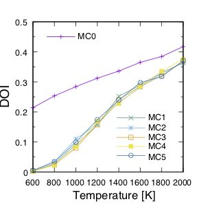
This process can be calculated by repeating AL.sh and MC.sh in turn. The actual result of the calculation of the inversion rate (DOI) is shown in the figure below. In this example, the first result is MC0, followed by MC1, MC2, and so on. The first run is quite different from the others, thus we can expect that it is not accurate. On the other hand, if we train on the results of one Monte Carlo run, we find that the values are almost identical from the next run.

The DOI can be calculated by the following procedure.

1. Go to MCxxx directory.

2. Create Tseparate directory by srun -n 8 abicsRXsepT ../input.toml. (The number of processes should be the same as the number of replicas for abics_sampling. In this tutorial, the number of parallelism is set to 8, so set it to 8.)

3. copy calc_DOI.py and MgAl2O4.vasp in the sample directory.

4. Calculate the degree of inversion for each temperature by srun -n 8 python3 calc_DOI.py ../input.toml. (Align with the number of parallelism when abics_sampling is executed. In this tutorial, the number of parallelism is set to 8, so set it to 8.)

In general, you will need to write your own scripts (calc_DOI.py in the current example) for calculating thermodynamic averages from the structures accumulated for each temperature in MCxxx/Tseparate.

Also, please note that the number of Monte Carlo steps in this example input is not enough for fully converging the degree of inversion. It is recommended to perform a separate RXMC calculation using the obtained neural network model with a larger number of sampling steps to calculate thermodynamic averages.

4.2.3. Predict energy of annet model via LAMMPS interface

abICS can call the aenet library via the LAMMPS interface (aenetPyLammps). This is faster than calling aenet directly because it does not need file I/O. The set of input files used in this tutorial can be found in examples/active_learning_qe.

Install aenetPyLammps

To use aenetPyLammps, you need to install aenet-lammps and lammps.

• URL : https://github.com/HidekiMori-CIT/aenet-lammps

• Use the commit 5d0f4bca .

  • git checkout 5d0f4bca

• Please install aenet-lammps` according to the procedure specified in the above URL. Below are notes on installation.

  • aenet

    • Make sure to add -fPIC to FCFLAGS in makefiles/Makefile.*.

  • lammps

    • Make sure to add LMP_INC = -DLAMMPS_EXCEPTIONS in src/Makefile.

    • Make sure to add mode=shared to the make command option as make mode=shared mpi (when GCC, for example).

  • After completing the above installation, run make install-python.

    • lammps python package will be installed to the Python environment which is invoked by python command.

Training

The training procedure is the same as the previous section.

Sampling

Input file for prediction

Instead of the input file predict.in for predict.x, place the input file in.lammps under the predict:

pair_style      aenet
pair_coeff      * * v00 Al Mg 15t-15t.nn Al Mg
neighbor        0.1 bin

The detailed format of in.lammmps is written in the README of aenet-lammps repository.

Input for Sampling

Change the type and run_scheme in the [sampling.solver] section of the input file to 'aenetPyLammps' and 'function', respectively.

[sampling.solver]
type = 'aenetPyLammps'
base_input_dir = ['./baseinput']
perturb = 0.0
run_scheme = 'function'