This jupyter notebook file is available at ISSP Data Repository (develop branch).
Gaussian process
PHYSBO performs Bayesian optimization while running Gaussian process regression.
Therefore, it is possible to run Gaussian process regression given training data, and to predict test data using the trained model.
In this section, the procedure is introduced.
[1]:
import numpy as np
import matplotlib.pyplot as plt
import physbo
Preparation of search candidate data
In this tutorial, the problem of finding a stable interface structure for Cu is used as an example. The values that have already been evaluated are used, although the evaluation of the objective function, i.e., the structural relaxation calculation, actually takes on the order of several hours per calculation. For more information on the problem setup, please refer to the following references
Kiyohara, H. Oda, K. Tsuda and T. Mizoguchi, “Acceleration of stable interface structure searching using a kriging approach”, Jpn. J. Appl. Phys. 55, 045502 (2016).
Save the dataset file s5-210.csv and load dataset from this file as the following:
[2]:
def load_data():
    A = np.asarray(np.loadtxt("s5-210.csv", skiprows=1, delimiter=","))
    X = A[:, 0:3]
    t = -A[:, 3]
    return X, t


X, t = load_data()
X = physbo.misc.centering(X)
Defining training data
A randomly selected 10% of the target data will be used as training data, and another randomly selected 10% will be used as test data.
[3]:
np.random.seed(12345)
N = len(t)
Ntrain = int(N * 0.1)
Ntest = min(int(N * 0.1), N - Ntrain)

id_all = np.random.choice(N, N, replace=False)
id_train = id_all[0:Ntrain]
id_test = id_all[Ntrain : Ntrain + Ntest]

X_train = X[id_train]
X_test = X[id_test]

t_train = t[id_train]
t_test = t[id_test]

print("Ntrain =", Ntrain)
print("Ntest =", Ntest)
Ntrain = 1798
Ntest = 1798
Learning and Prediction of Gaussian Processes
The following process is used to learn the Gaussian process and predict the test data.
Generate a model of the Gaussian process
The model is trained using X_train (parameters of the training data) and t_train (objective function value of the training data).
Run predictions on the test data (X_test) using the trained model.
Definition of covariance (Gaussian)
[4]:
cov = physbo.gp.cov.Gauss(X_train.shape[1], ard=False)
Definition of mean value
[5]:
mean = physbo.gp.mean.Const()
Definition of likelihood function (Gaussian)
[6]:
lik = physbo.gp.lik.Gauss()
Generation of a Gaussian Process Model
[7]:
gp = physbo.gp.Model(lik=lik, mean=mean, cov=cov)
config = physbo.misc.SetConfig()
Learning a Gaussian process model.
[8]:
gp.fit(X_train, t_train, config)
Start the initial hyper parameter searching ...
Done

Start the hyper parameter learning ...
0 -th epoch marginal likelihood 16183.326658360042
50 -th epoch marginal likelihood 3766.734249925179
100 -th epoch marginal likelihood 1450.3500890285495
150 -th epoch marginal likelihood 127.98987541463339
200 -th epoch marginal likelihood -665.714179830029
250 -th epoch marginal likelihood -1132.4472253356018
300 -th epoch marginal likelihood -1340.5546244777697
350 -th epoch marginal likelihood -1438.398304111003
400 -th epoch marginal likelihood -1464.575163347392
450 -th epoch marginal likelihood -1478.4817552781674
500 -th epoch marginal likelihood -1485.7013807794137
Done
Output the parameters in the learned Gaussian process.
[9]:
gp.print_params()
likelihood parameter =   [-2.44630277]
mean parameter in GP prior:  [-1.06536273]
covariance parameter in GP prior:  [-0.64183368 -2.49190006]
Calculating the mean (predicted value) and variance of the test data
[10]:
gp.prepare(X_train, t_train)
fmean = gp.get_post_fmean(X_train, X_test)
fcov = gp.get_post_fcov(X_train, X_test)
Results of prediction
[11]:
fmean
[11]:
array([-1.04749842, -0.99756623, -1.09935748, ..., -1.07561436,
       -1.07684287, -1.10315271], shape=(1798,))
Results of covariance
[12]:
fcov
[12]:
array([0.0006267 , 0.00053271, 0.00095938, ..., 0.00067901, 0.00066522,
       0.00055919], shape=(1798,))
Output mean square error of prediction
[13]:
np.mean((fmean - t_test) ** 2)
[13]:
np.float64(0.006925305425496946)
A simple metric to investigate how important each feature is in the obtained regression model is permutation importance (PI). In PHYSBO, this can be calculated using the get_permutation_importance function.
[14]:
pi_mean, pi_std = gp.get_permutation_importance(X_train, t_train, n_perm=100)
[15]:
features = list(range(len(pi_mean)))

plt.figure(figsize=(8, 5))
plt.barh(
    features,
    pi_mean,
    xerr=pi_std,
)
plt.gca().invert_yaxis()
plt.yticks(features)
plt.xlabel("Permutation Importance")
plt.ylabel("Feature")
plt.tight_layout()
# print("save permutation_importance.pdf")
# plt.savefig("permutation_importance.pdf")
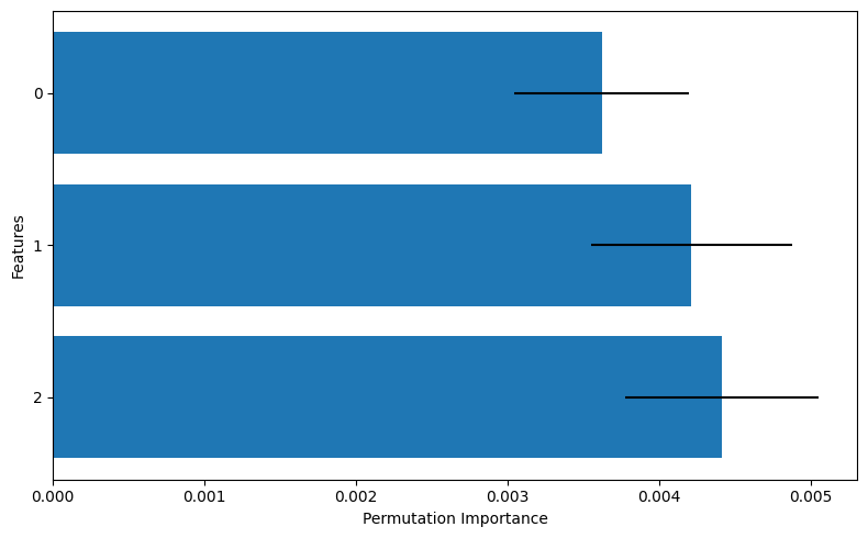
In this graph, the bar chart represents the mean value of the permutation importance (PI), while the line segments indicate the standard deviation. From this, we can interpret that features 1 and 2 appear to be more important compared to feature 0.
Not only gp.model, but policy also has the get_permutation_importance function. The usage is policy.get_permutation_importance(n_perm). In the case of policy, PI is calculated based on the stored training data, so unlike model, there is no need to pass the data again.
Prediction by trained models
Read the parameters of the trained model as gp_params and make predictions using them.
By storing gp_params and training data (X_train, t_train), prediction by the trained model is possible.
Prepare the learned parameters (must be done immediately after learning)
[16]:
# Prepare the learned parameters as a 1D array
gp_params = np.append(
    np.append(gp.lik.params, gp.prior.mean.params), gp.prior.cov.params
)

gp_params
[16]:
array([-2.44630277, -1.06536273, -0.64183368, -2.49190006])
Prepare a model similar to the one used for training as gp
[17]:
# Definition of covariance (Gaussian)
cov = physbo.gp.cov.Gauss(X_train.shape[1], ard=False)

# Definition of mean value
mean = physbo.gp.mean.Const()

# Definition of likelihood function (Gaussian)
lik = physbo.gp.lik.Gauss()

# Generation of a Gaussian Process Model
gp = physbo.gp.Model(lik=lik, mean=mean, cov=cov)
Prepare a model similar to the one used for training as gp
[18]:
# Input learned parameters into the Gaussian process.
gp.set_params(gp_params)

# Calculate the mean (predicted value) and variance of the test data
gp.prepare(X_train, t_train)
fmean = gp.get_post_fmean(X_train, X_test)
fcov = gp.get_post_fcov(X_train, X_test)
Results of prediction
[19]:
fmean
[19]:
array([-1.04749842, -0.99756623, -1.09935748, ..., -1.07561436,
       -1.07684287, -1.10315271], shape=(1798,))
Results of covariance
[20]:
fcov
[20]:
array([0.0006267 , 0.00053271, 0.00095938, ..., 0.00067901, 0.00066522,
       0.00055919], shape=(1798,))
Output mean square error of prediction
[21]:
np.mean((fmean - t_test) ** 2)
[21]:
np.float64(0.006925305425496946)
Bayesian linear regression with random feature map
PHYSBO also provides Bayesian linear model with random feature map for acceleration of prediction (for details, see Algorithm). It is convenient to construct Bayesian linear model blm from trained Gaussian process model gp.
[22]:
# number of random features
M = 100

# Define blm model from gp
blm = gp.export_blm(M)

# Initializes model by using the first training dataset
blm.prepare(X_train, t_train)
Calculates posterior mean of weights
[23]:
blm.get_post_params_mean()
Calculates posterior mean of model (function)
[24]:
blm.get_post_fmean(X_test)
[24]:
array([-1.00281987, -1.021285  , -1.05703224, ..., -1.03903166,
       -1.05308985, -1.0886392 ], shape=(1798,))
Draws samples of weights
[25]:
blm.sampling(N)
[25]:
array([17982.25182061, 17982.02571459, 17981.80194809, 17982.25510674,
       17981.66362023, 17981.94995566, 17981.64584662, 17981.6419771 ,
       17982.60806258, 17982.35413272, 17981.80628787, 17981.86662535,
       17981.7296249 , 17982.36710795, 17982.0886057 , 17982.35419747,
       17981.62999812, 17981.84312661, 17981.99848416, 17981.89540307,
       17982.11222119, 17983.94507764, 17982.5092398 , 17982.24701584,
       17982.32421083, 17982.13933822, 17982.02862381, 17982.20436152,
       17981.96314564, 17981.20549811, 17981.89276456, 17981.90269375,
       17982.19008124, 17982.3800117 , 17981.66267877, 17982.97578728,
       17981.75381325, 17981.6304626 , 17982.98456174, 17981.95586776,
       17982.09232995, 17981.79500226, 17981.16359087, 17981.92477529,
       17982.41587154, 17982.37029713, 17981.98737483, 17982.08471758,
       17982.10916536, 17981.61480804, 17981.52740076, 17981.503297  ,
       17982.2895881 , 17982.05691979, 17982.33931683, 17981.76721548,
       17982.3620971 , 17982.5609712 , 17982.35823842, 17981.90810384,
       17981.9280631 , 17982.15268503, 17981.98441024, 17981.65256567,
       17981.56620624, 17981.73128853, 17981.82886044, 17982.77982802,
       17980.24044025, 17982.2722357 , 17981.61547109, 17982.33799225,
       17981.56915725, 17981.90126661, 17982.9278042 , 17982.05524349,
       17982.37014053, 17982.19934487, 17982.00357933, 17982.1214092 ,
       17981.90573108, 17982.08097159, 17981.20791008, 17982.38033984,
       17981.68701063, 17981.73791397, 17981.35117105, 17982.45506255,
       17982.12698395, 17981.41256826, 17981.38139235, 17981.99369549,
       17981.85706449, 17982.11788584, 17981.8681819 , 17981.98174068,
       17981.60341704, 17982.26672048, 17980.97479345, 17981.95121096])
Draws samples from model
[26]:
blm.predict_sampling(X_test)
[26]:
array([[-1.08420802, -1.04279261, -1.08889251, ..., -1.16072789,
        -1.00383682, -1.05860927]], shape=(1, 1798))
Calculates posterior covariance of model
[27]:
blm.get_post_fcov(X_test)
[27]:
array([0.00027617, 0.00024492, 0.00041572, ..., 0.000287  , 0.00032018,
       0.000251  ], shape=(1798,))
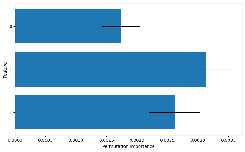
Calculate the permutation importance using get_permutation_importance function.
[28]:
import matplotlib.pyplot as plt

pi_mean, pi_std = blm.get_permutation_importance(X_train, t_train, n_perm=100)
features = list(range(len(pi_mean)))

plt.figure(figsize=(8, 5))
plt.barh(
    features,
    pi_mean,
    xerr=pi_std,
)
plt.gca().invert_yaxis()
plt.yticks(features)
plt.xlabel("Permutation Importance")
plt.ylabel("Feature")
plt.tight_layout()
Notes
In this tutorial, we made predictions using the same \(X\) values that were registered beforehand. If you wish to make predictions for new parameters \(X_\text{new}\) that are not included in \(X\) using the trained model, you should first compute the mean (\(X_\text{mean}\)) and standard deviation (\(X_\text{std}\)) of the training data \(X\), and then transform your new data as follows:
\(X_\text{new} = (X_\text{new} - X_\text{mean}) / X_\text{std}\)
This transformation allows your model to make accurate predictions for \(X_\text{new}\). Also, note that the data you pass should be in the form of an ndarray. Therefore, if \(X_\text{new}\) is a single data point, it needs to be converted beforehand. For example, if \(X_\text{new}\) is a scalar value, you should convert it as: X_new = np.array(X_new).reshape(1) or in a similar way before passing it to the model.