This jupyter notebook file is available at ISSP Data Repository (develop branch).
Basic usage of PHYSBO
Introduction
In this tutorial, we will learn how to use PHYSBO to solve a optimization problem.
First, we import modules.
[1]:
import numpy as np
import matplotlib.pyplot as plt
import physbo
The problem we will solve is to find the minimum value of the one-dimensional function \(f(x) = 3 x^4 + 4 x ^3 + 1.0\). The exact solution is \(x=-1.0\).
[2]:
def fn(x):
    return 3 * x**4 + 4 * x**3 + 1.0
Defining the search space
Define the search space for the function to be optimized. In PHYSBO, you need to prepare the candidate points to be searched in advance as a np.ndarray. The array shape should be (N, d), where N is the number of candidate points and d is the dimensionality of the search space. If you want to divide each dimension into equally spaced intervals, you can conveniently use physbo.search.utility.make_grid. In the example below, the search space X is defined by splitting the
interval from x_min = -2.0 to x_max = 2.0 into window_num=10001 evenly spaced grid points.
[3]:
window_num=10001
x_max = [2.0]
x_min = [-2.0]

X = physbo.search.utility.make_grid(x_min, x_max, window_num)
Definition of the simulator
In PHYSBO, the function (or Callable object) that actually computes the objective function is called the simulator.
The simulator receives an index or indices (action) of candidate points to evaluate and returns the value(s) of the objective function at those points. Typically, to allow evaluation of multiple points at once, action is expected to be a np.ndarray of indices.
Since PHYSBO always tries to maximize the objective function, for minimization problems like this example, we simply return the negative value of the function to turn it into a maximization problem.
You can easily create such a simulator using physbo.search.utility.Simulator, which wraps your function and candidate points to meet these requirements.
[4]:
simulator = physbo.search.utility.Simulator(X, fn, negate=True)
Performing optimization
Setting policy
First, set the optimization Policy.
Next, set test_X to the matrix of search candidates (numpy.array).
[5]:
# set policy
policy = physbo.search.discrete.Policy(test_X=X)

# set seed
policy.set_seed(0)
When policy is set, no optimization is done yet. Execute the following methods on policy to optimize it.
random_search.bayes_search.
If you specify the simulator and the number of search steps in these methods, the following loop will be executed for the number of search steps.
Select the next parameter to be executed from the candidate parameters.
Execute
simulatorwith the selected parameters.
The default number of parameter returned by i) is one, but it is possible to return multiple parameters in one step. See the section “Searching for multiple candidates at once” for details.
Also, instead of running the above loop inside PHYSBO, it is possible to control i) and ii) separately from the outside. In other words, it is possible to propose the next parameter to be executed from PHYSBO, evaluate its objective function value in some way outside PHYSBO (e.g., by experiment rather than numerical calculation), propose it in some way outside PHYSBO, and register the evaluated value in PHYSBO. For more details, please refer to the “Running Interactively” section of the tutorial.
Random Search
First of all, let’s perform a random search.
Since Bayesian optimization requires at least two objective function values to be obtained (the initial number of data required depends on the problem to be optimized and the dimension d of the parameters), we will first perform a random search.
argument.
max_num_probes: Number of search steps.simulator: The simulator of the objective function (an object of class simulator).
[6]:
res = policy.random_search(max_num_probes=20, simulator=simulator)
0001-th step: f(x) = -51.387604 (action=9395)
   current best f(x) = -51.387604 (best action=9395)

0002-th step: f(x) = -0.581263 (action=3583)
   current best f(x) = -0.581263 (best action=3583)

0003-th step: f(x) = -0.827643 (action=4015)
   current best f(x) = -0.581263 (best action=3583)

0004-th step: f(x) = -14.220707 (action=154)
   current best f(x) = -0.581263 (best action=3583)

0005-th step: f(x) = -34.192764 (action=8908)
   current best f(x) = -0.581263 (best action=3583)

0006-th step: f(x) = -31.595527 (action=8819)
   current best f(x) = -0.581263 (best action=3583)

0007-th step: f(x) = -0.361729 (action=3269)
   current best f(x) = -0.361729 (best action=3269)

0008-th step: f(x) = -0.755839 (action=3870)
   current best f(x) = -0.361729 (best action=3269)

0009-th step: f(x) = -10.883996 (action=370)
   current best f(x) = -0.361729 (best action=3269)

0010-th step: f(x) = -0.150313 (action=2949)
   current best f(x) = -0.150313 (best action=2949)

0011-th step: f(x) = -3.885764 (action=6926)
   current best f(x) = -0.150313 (best action=2949)

0012-th step: f(x) = -3.525070 (action=6851)
   current best f(x) = -0.150313 (best action=2949)

0013-th step: f(x) = -3.252476 (action=6789)
   current best f(x) = -0.150313 (best action=2949)

0014-th step: f(x) = -7.524212 (action=641)
   current best f(x) = -0.150313 (best action=2949)

0015-th step: f(x) = -16.136719 (action=8125)
   current best f(x) = -0.150313 (best action=2949)

0016-th step: f(x) = -1.439937 (action=6090)
   current best f(x) = -0.150313 (best action=2949)

0017-th step: f(x) = -9.415991 (action=480)
   current best f(x) = -0.150313 (best action=2949)

0018-th step: f(x) = -4.854365 (action=925)
   current best f(x) = -0.150313 (best action=2949)

0019-th step: f(x) = -1.042368 (action=5523)
   current best f(x) = -0.150313 (best action=2949)

0020-th step: f(x) = -19.075990 (action=8288)
   current best f(x) = -0.150313 (best action=2949)
When executed, the objective function value and its action ID for each step, and the best value up to now and its action ID will be printed as follows.
0020-th step: f(x) = -19.075990 (action=8288)
   current best f(x) = -0.150313 (best action=2949)
These output can be suppressed by setting is_disp=False in the argument.
Bayesian Optimization
Next, we run the Bayesian optimization as follows.
argument.
max_num_probes: Number of search steps.simulator: The simulator of the objective function (an object of class simulator).score: The type of acquisition function. You can specify one of the followingTS (Thompson Sampling)
EI (Expected Improvement)
PI (Probability of Improvement)
interval: The hyperparameters are trained at the specified interval. If a negative value is specified, no hyperparameter will be learned. 0 means that hyperparameter learning will be performed only in the first step.num_rand_basis: Number of basis functions. 0 means that a normal Gaussian process without Bayesian linear model will be used.
[7]:
res = policy.bayes_search(
    max_num_probes=50,
    simulator=simulator,
    score="TS",
    interval=0,
    num_rand_basis=500,
    is_disp=False,
)
Checking the results
res is returned as an object of the history class (physbo.search.discrete.results.history).res.fx: The history of evaluated values of simulator (objective function).res.chosen_actions: The history of action IDs (parameters) when the simulator was evaluated.fbest, best_action= res.export_all_sequence_best_fx(): The history of best values and their action IDs (parameters) for all timings when the simulator was evaluated.res.total_num_search: Total number of simulator evaluations.
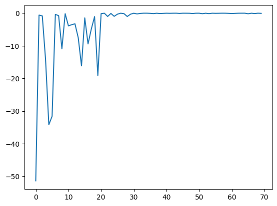
res.fx and best_fx should range up to res.total_num_search, respectively.[8]:
plt.plot(res.fx[0:res.total_num_search])
[8]:
[<matplotlib.lines.Line2D at 0x11481bd10>]
[9]:
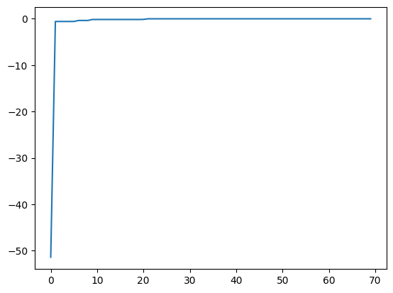
best_fx, best_action = res.export_all_sequence_best_fx()
plt.plot(best_fx)
[9]:
[<matplotlib.lines.Line2D at 0x11486bc90>]
Serializing the results
The search results can be saved to an external file using the save method.
[10]:
res.save('search_result.npz')
[11]:
del res
Load the saved result file as follows:
[12]:
res = physbo.search.discrete.History()
res.load('search_result.npz')
Finally, the candidate with the best score can be displayed as follows. You can see that we have arrived at the correct solution \(x=-1\).
[13]:
print(X[int(best_action[-1])])
[-1.002]
Prediction
policy serves get_post_fmean and get_post_fcov methods for calculating mean value and variance of Gaussian process (post distribution).
[14]:
mean = policy.get_post_fmean(X)
var = policy.get_post_fcov(X)
std = np.sqrt(var)
xs = X[:,0]

ax = plt.subplot()
ax.plot(xs, mean)
ax.fill_between(xs, mean-std, mean+std, color="blue", alpha=.1)
[14]:
<matplotlib.collections.FillBetweenPolyCollection at 0x114342610>
Acquisition function
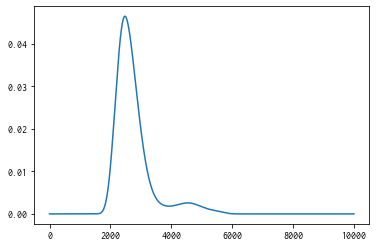
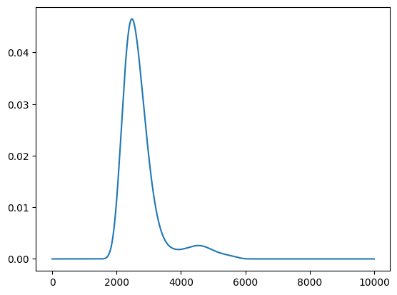
policy serves get_score method for calculating acquisition function.
[15]:
scores = policy.get_score(mode="EI", xs=X)
plt.plot(scores)
[15]:
[<matplotlib.lines.Line2D at 0x114967c10>]
Parallelization
PHYSBO can calculate acquisition functions for candidates in parallel by using MPI via mpi4py . To enable MPI parallelization, pass a MPI communicator such as MPI.COMM_WORLD to a keyword argument, comm of the constructor of the policy.
[16]:
# from mpi4py import MPI
# policy = physbo.search.discrete.policy(test_X=X, comm=MPI.COMM_WORLD)