This jupyter notebook file is available at ISSP Data Repository (develop branch).

Search multiple candidates at once

This is a tutorial for evaluating two or more candidates at once in a single search step.

import numpy as np
import matplotlib.pyplot as plt
import physbo

Prepare the search candidate data

As the previous tutorials, save the dataset file s5-210.csv and load dataset from this file as the following:

def load_data():
    A =  np.asarray(np.loadtxt('s5-210.csv',skiprows=1, delimiter=',') )
    X = A[:,0:3]
    t  = -A[:,3]
    return X, t

X, t = load_data()
X = physbo.misc.centering(X)

Definition of simulator

class Simulator:
    def __init__(self, t):
        self.t = t

    def __call__( self, action ):
        return self.t[action]

simulator = Simulator(t)

# Example of running the simulator
simulator([1,12,123])

array([-1.01487066, -1.22884748, -1.05572838])

Performing optimizations

# set policy
policy = physbo.search.discrete.Policy(test_X=X)

# set seed
policy.set_seed( 0 )

num_search_each_probe allows you to specify the number of candidates to evaluate in each search step.

In the following example, the simulator will be evaluated 2 × 10 = 20 times by random search and 8 × 10 = 80 times by Bayesian optimization.

argument.

• max_num_probes: Number of search steps.

• num_search_each_probe: Number of candidates to evaluate at each search step.

res = policy.random_search(
    max_num_probes=2, num_search_each_probe=10, simulator=simulator
)

res = policy.bayes_search(
    max_num_probes=8,
    num_search_each_probe=10,
    simulator=simulator,
    score="EI",
    interval=2,
    num_rand_basis=100,
)

0001-th multiple probe search (random)
current best f(x) = -0.980054 (best action = 4547)
list of simulation results
f(x)=-1.070602 (action = 15673)
f(x)=-1.009056 (action = 9559)
f(x)=-1.195844 (action = 16927)
f(x)=-0.980054 (action = 4547)
f(x)=-0.992820 (action = 2553)
f(x)=-1.146676 (action = 13144)
f(x)=-1.006255 (action = 10827)
f(x)=-0.999862 (action = 1995)
f(x)=-1.055445 (action = 10763)
f(x)=-1.100970 (action = 16450)


0002-th multiple probe search (random)
current best f(x) = -0.980054 (best action = 4547)
list of simulation results
f(x)=-1.208666 (action = 13085)
f(x)=-1.069404 (action = 15133)
f(x)=-1.031642 (action = 1706)
f(x)=-1.016702 (action = 2464)
f(x)=-1.172569 (action = 17812)
f(x)=-1.082219 (action = 16533)
f(x)=-1.025272 (action = 1336)
f(x)=-1.031761 (action = 10076)
f(x)=-0.984972 (action = 8876)
f(x)=-1.107730 (action = 15577)


Start the initial hyper parameter searching ...
Done

Start the hyper parameter learning ...
0 -th epoch marginal likelihood -22.83973847978998
50 -th epoch marginal likelihood -24.17761713990829
100 -th epoch marginal likelihood -24.831018285821855
150 -th epoch marginal likelihood -25.15416148652374
200 -th epoch marginal likelihood -25.33446562798866
250 -th epoch marginal likelihood -25.455155010625035
300 -th epoch marginal likelihood -25.550091453614574
350 -th epoch marginal likelihood -25.63130127933855
400 -th epoch marginal likelihood -25.70238745744905
450 -th epoch marginal likelihood -25.764347677344432
500 -th epoch marginal likelihood -25.817697844806304
Done

0003-th multiple probe search (EI)
current best f(x) = -0.963125 (best action = 7028)
list of simulation results
f(x)=-0.999831 (action = 8311)
f(x)=-0.971324 (action = 7695)
f(x)=-1.022353 (action = 11640)
f(x)=-2.231758 (action = 2989)
f(x)=-1.330630 (action = 14999)
f(x)=-1.490831 (action = 8998)
f(x)=-0.963461 (action = 8382)
f(x)=-1.006954 (action = 1144)
f(x)=-1.072227 (action = 8240)
f(x)=-0.963125 (action = 7028)


0004-th multiple probe search (EI)
current best f(x) = -0.963125 (best action = 7028)
list of simulation results
f(x)=-1.020075 (action = 2308)
f(x)=-1.013442 (action = 14800)
f(x)=-1.021923 (action = 2271)
f(x)=-1.008847 (action = 2272)
f(x)=-1.011485 (action = 2235)
f(x)=-1.124811 (action = 15021)
f(x)=-1.019125 (action = 2345)
f(x)=-1.034768 (action = 2344)
f(x)=-1.509526 (action = 15013)
f(x)=-1.007610 (action = 14763)


Start the initial hyper parameter searching ...
Done

Start the hyper parameter learning ...
0 -th epoch marginal likelihood 23.073628205443782
50 -th epoch marginal likelihood 9.719167854722315
100 -th epoch marginal likelihood 1.4617496079117132
150 -th epoch marginal likelihood -3.798836012927623
200 -th epoch marginal likelihood -7.323789523166454
250 -th epoch marginal likelihood -9.785789330036504
300 -th epoch marginal likelihood -11.56593442759742
350 -th epoch marginal likelihood -12.890764162978456
400 -th epoch marginal likelihood -13.902281570598056
450 -th epoch marginal likelihood -14.693902339866337
500 -th epoch marginal likelihood -15.329257712391108
Done

0005-th multiple probe search (EI)
current best f(x) = -0.963125 (best action = 7028)
list of simulation results
f(x)=-1.065906 (action = 6464)
f(x)=-1.016857 (action = 9064)
f(x)=-1.052785 (action = 17091)
f(x)=-1.091519 (action = 14954)
f(x)=-0.984545 (action = 7141)
f(x)=-0.994764 (action = 3492)
f(x)=-0.986965 (action = 6497)
f(x)=-1.059148 (action = 5)
f(x)=-1.062454 (action = 16945)
f(x)=-1.076059 (action = 677)


0006-th multiple probe search (EI)
current best f(x) = -0.963125 (best action = 7028)
list of simulation results
f(x)=-0.990597 (action = 1590)
f(x)=-1.076706 (action = 13246)
f(x)=-1.145412 (action = 16280)
f(x)=-0.995306 (action = 11877)
f(x)=-1.023616 (action = 11106)
f(x)=-1.052131 (action = 11400)
f(x)=-0.991510 (action = 1627)
f(x)=-1.227426 (action = 6008)
f(x)=-0.965286 (action = 4587)
f(x)=-1.060802 (action = 13209)


Start the initial hyper parameter searching ...
Done

Start the hyper parameter learning ...
0 -th epoch marginal likelihood 473.6562814170836
50 -th epoch marginal likelihood 363.6169713454166
100 -th epoch marginal likelihood 280.4346034309093
150 -th epoch marginal likelihood 218.0054785862581
200 -th epoch marginal likelihood 170.65000562578436
250 -th epoch marginal likelihood 134.22268953329905
300 -th epoch marginal likelihood 105.78132811282859
350 -th epoch marginal likelihood 83.25038707552301
400 -th epoch marginal likelihood 65.15788635125642
450 -th epoch marginal likelihood 50.44852382153766
500 -th epoch marginal likelihood 38.35577038115986
Done

0007-th multiple probe search (EI)
current best f(x) = -0.960321 (best action = 8213)
list of simulation results
f(x)=-1.057612 (action = 14984)
f(x)=-0.990722 (action = 10878)
f(x)=-0.963464 (action = 8250)
f(x)=-1.043198 (action = 14947)
f(x)=-0.983485 (action = 10915)
f(x)=-0.968059 (action = 8287)
f(x)=-1.059552 (action = 14983)
f(x)=-0.999771 (action = 10841)
f(x)=-0.960321 (action = 8213)
f(x)=-0.977957 (action = 10952)


0008-th multiple probe search (EI)
current best f(x) = -0.960321 (best action = 8213)
list of simulation results
f(x)=-0.995292 (action = 703)
f(x)=-0.983678 (action = 8968)
f(x)=-0.997529 (action = 8967)
f(x)=-0.999770 (action = 666)
f(x)=-0.992400 (action = 740)
f(x)=-1.014959 (action = 4879)
f(x)=-0.977174 (action = 11967)
f(x)=-1.005922 (action = 629)
f(x)=-1.013689 (action = 592)
f(x)=-0.972775 (action = 8969)


Start the initial hyper parameter searching ...
Done

Start the hyper parameter learning ...
0 -th epoch marginal likelihood 70.33429991441128
50 -th epoch marginal likelihood 28.7644910600593
100 -th epoch marginal likelihood 0.4848519552564312
150 -th epoch marginal likelihood -18.236558043785692
200 -th epoch marginal likelihood -32.06535289863197
250 -th epoch marginal likelihood -42.7681819466728
300 -th epoch marginal likelihood -51.46052158149965
350 -th epoch marginal likelihood -56.687714339736516
400 -th epoch marginal likelihood -61.70347758865685
450 -th epoch marginal likelihood -65.19178853027779
500 -th epoch marginal likelihood -68.0555175525907
Done

0009-th multiple probe search (EI)
current best f(x) = -0.960321 (best action = 8213)
list of simulation results
f(x)=-1.055798 (action = 985)
f(x)=-0.997708 (action = 3033)
f(x)=-1.038770 (action = 1614)
f(x)=-1.031694 (action = 652)
f(x)=-1.033686 (action = 1207)
f(x)=-1.036349 (action = 763)
f(x)=-1.033301 (action = 1688)
f(x)=-1.045945 (action = 3133)
f(x)=-1.052235 (action = 947)
f(x)=-1.040833 (action = 430)


0010-th multiple probe search (EI)
current best f(x) = -0.960321 (best action = 8213)
list of simulation results
f(x)=-2.497328 (action = 17945)
f(x)=-0.990424 (action = 1480)
f(x)=-0.991675 (action = 5957)
f(x)=-0.990406 (action = 1517)
f(x)=-0.990488 (action = 1443)
f(x)=-1.094922 (action = 17908)
f(x)=-1.058552 (action = 3766)
f(x)=-1.053202 (action = 3803)
f(x)=-1.110345 (action = 15737)
f(x)=-0.990559 (action = 1554)

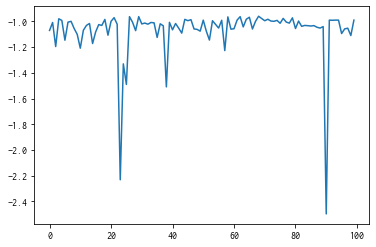
Checking results

plt.plot(res.fx[0:res.total_num_search])

[<matplotlib.lines.Line2D at 0x11311cf10>]

best_fx, best_action = res.export_all_sequence_best_fx()
plt.plot(best_fx)

[<matplotlib.lines.Line2D at 0x115096190>]

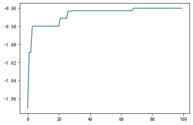
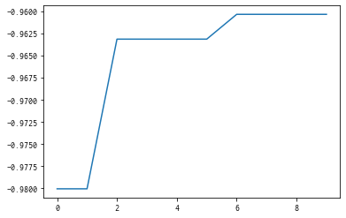
With res.export_sequence_best_fx(), you can get the best value obtained at each step and the history of the action.

The difference between res.export_all_sequence_best_fx() and res.export_all_sequence_best_fx() is that the information is not for each evaluation of the simulator, but for each search step. In this case, the total number of steps is 10, and the number of evaluations is 100.

best_fx, best_action = res.export_sequence_best_fx()
plt.plot(best_fx)

[<matplotlib.lines.Line2D at 0x1150a2510>]