This jupyter notebook file is available at ISSP Data Repository (v3.0.0 branch).

Gaussian process

PHYSBO performs Bayesian optimization while running Gaussian process regression.

Therefore, it is possible to run Gaussian process regression given training data, and to predict test data using the trained model.

In this section, the procedure is introduced.

Preparation of search candidate data

In this tutorial, the problem of finding a stable interface structure for Cu is used as an example. The values that have already been evaluated are used, although the evaluation of the objective function, i.e., the structural relaxation calculation, actually takes on the order of several hours per calculation. For more information on the problem setup, please refer to the following references

• 19. Kiyohara, H. Oda, K. Tsuda and T. Mizoguchi, “Acceleration of stable interface structure searching using a kriging approach”, Jpn. J. Appl. Phys. 55, 045502 (2016).

Save the dataset file s5-210.csv and load dataset from this file as the following:

import numpy as np
import matplotlib.pyplot as plt

import physbo


def load_data():
    A =  np.asarray(np.loadtxt('s5-210.csv',skiprows=1, delimiter=',') )
    X = A[:,0:3]
    t  = -A[:,3]
    return X, t

X, t = load_data()
X = physbo.misc.centering( X )

Cythonized version of physbo is used

Defining training data

A randomly selected 10% of the target data will be used as training data, and another randomly selected 10% will be used as test data.

N = len(t)
Ntrain = int(N*0.1)
Ntest = min(int(N*0.1), N-Ntrain)

id_all   = np.random.choice(N, N, replace=False)
id_train  = id_all[0:Ntrain]
id_test = id_all[Ntrain:Ntrain+Ntest]

X_train = X[id_train]
X_test = X[id_test]

t_train = t[id_train]
t_test = t[id_test]

print("Ntrain =", Ntrain)
print("Ntest =", Ntest)

Ntrain = 1798
Ntest = 1798

Learning and Prediction of Gaussian Processes

The following process is used to learn the Gaussian process and predict the test data.

1. Generate a model of the Gaussian process

2. The model is trained using X_train (parameters of the training data) and t_train (objective function value of the training data).

3. Run predictions on the test data (X_test) using the trained model.

Definition of covariance (Gaussian)

cov = physbo.gp.cov.Gauss( X_train.shape[1],ard = False )

Definition of mean value

mean = physbo.gp.mean.Const()

Definition of likelihood function (Gaussian)

lik = physbo.gp.lik.Gauss()

Generation of a Gaussian Process Model

gp = physbo.gp.Model(lik=lik,mean=mean,cov=cov)
config = physbo.misc.SetConfig()

Learning a Gaussian process model.

gp.fit(X_train, t_train, config)

Start the initial hyper parameter searching ...
Done

Start the hyper parameter learning ...
0 -th epoch marginal likelihood 14215.691923517237
50 -th epoch marginal likelihood 3693.9141289009012
100 -th epoch marginal likelihood 1669.6612412198328
150 -th epoch marginal likelihood 616.2890017670807
200 -th epoch marginal likelihood -390.0794868410685
250 -th epoch marginal likelihood -1079.3135563326973
300 -th epoch marginal likelihood -1605.0063300177012
350 -th epoch marginal likelihood -1845.6167857237276
400 -th epoch marginal likelihood -1999.6781455787882
450 -th epoch marginal likelihood -2058.0614082304874
500 -th epoch marginal likelihood -2119.872337999709
Done

Output the parameters in the learned Gaussian process.

gp.print_params()

likelihood parameter =   [-3.03559485]
mean parameter in GP prior:  [-1.05829024]
covariance parameter in GP prior:  [-0.87638318 -2.59947926]

Calculating the mean (predicted value) and variance of the test data

gp.prepare(X_train, t_train)
fmean = gp.get_post_fmean(X_train, X_test)
fcov = gp.get_post_fcov(X_train, X_test)

Results of prediction

fmean

array([-1.00577644, -1.09101548, -0.98765945, ..., -1.10355396,
       -1.00772337, -1.16177325])

Results of covariance

fcov

array([0.00038442, 0.00043068, 0.00049836, ..., 0.00034837, 0.00037362,
       0.00064077])

Output mean square error of prediction

np.mean((fmean-t_test)**2)

0.003795862874772909

A simple metric to investigate how important each feature is in the obtained regression model is permutation importance (PI). In PHYSBO, this can be calculated using the get_permutation_importance function.

pi_mean, pi_std = gp.get_permutation_importance(X_train, t_train, n_perm=100)

features = list(range(len(pi_mean)))

plt.figure(figsize=(8, 5))
plt.barh(
    features,
    pi_mean,
    xerr=pi_std,
)
plt.gca().invert_yaxis()
plt.yticks(features)
plt.xlabel("Permutation Importance")
plt.ylabel("Features")
plt.tight_layout()
# print("save permutation_importance.pdf")
# plt.savefig("permutation_importance.pdf")

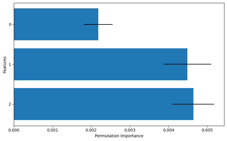
In this graph, the bar chart represents the mean value of the permutation importance (PI), while the line segments indicate the standard deviation. From this, we can interpret that features 1 and 2 appear to be more important compared to feature 0.

Not only gp.model, but policy also has the get_permutation_importance function. The usage is policy.get_permutation_importance(n_perm). In the case of policy, PI is calculated based on the stored training data, so unlike model, there is no need to pass the data again.

Prediction by trained models

Read the parameters of the trained model as gp_params and make predictions using them.

By storing gp_params and training data (X_train, t_train), prediction by the trained model is possible.

Prepare the learned parameters (must be done immediately after learning)

#Prepare the learned parameters as a 1D array
gp_params =  np.append(np.append(gp.lik.params, gp.prior.mean.params), gp.prior.cov.params)

gp_params

array([-3.03559485, -1.05829024, -0.87638318, -2.59947926])

Prepare a model similar to the one used for training as gp

#Definition of covariance (Gaussian)
cov = physbo.gp.cov.Gauss( X_train.shape[1],ard = False )

#Definition of mean value
mean = physbo.gp.mean.Const()

#Definition of likelihood function (Gaussian)
lik = physbo.gp.lik.Gauss()

#Generation of a Gaussian Process Model
gp = physbo.gp.Model(lik=lik,mean=mean,cov=cov)

Prepare a model similar to the one used for training as gp

#Input learned parameters into the Gaussian process.
gp.set_params(gp_params)


#Calculate the mean (predicted value) and variance of the test data
gp.prepare(X_train, t_train)
fmean = gp.get_post_fmean(X_train, X_test)
fcov = gp.get_post_fcov(X_train, X_test)

Results of prediction

fmean

array([-1.00577644, -1.09101548, -0.98765945, ..., -1.10355396,
       -1.00772337, -1.16177325])

Results of covariance

fcov

array([0.00038442, 0.00043068, 0.00049836, ..., 0.00034837, 0.00037362,
       0.00064077])

Output mean square error of prediction

np.mean((fmean-t_test)**2)

0.003795862874772909

Note: In the example above, we used the same pre-registered X to make predictions. If you want to make predictions for parameters X_new that is not included in X using the trained model, you first obtain the mean (X_{mean}) and standard deviation (X_{std}) of the data X and then normalize X_{new} by (X_{new} - X_{mean}) / X_{std}. Also, the data format for X is ndarray format. Therefore, if X_{new} is a single data, it must be transformed to ndarray format. For example, if X_{new} is a real number, you should replace X_new as X_new = np.array(X_new).reshape(1)