This jupyter notebook file is available at ISSP Data Repository (v3.0.0 branch).
Basic usage of PHYSBO
Introduction
In this tutorial, we will introduce how to define the simulator class and find the minimum value of a one-dimensional function using PHYSBO.
First, we will import PHYSBO.
[1]:
import physbo
Cythonized version of physbo is used
Defining the search space
In the following example, the search space X is defined as a grid chopped by window_num=10001 divisions from x_min = -2.0 to x_max = 2.0. Note that X must be in window_num x d ndarray format (d is the number of dimensions, in this case one). In this case, d is the number of dimensions, in this case two, so we use reshape to transform it.
[2]:
#In
import numpy as np
import scipy
import physbo
import itertools

#In
#Create candidate
window_num=10001
x_max = 2.0
x_min = -2.0

X = np.linspace(x_min,x_max,window_num).reshape(window_num, 1)
Defining the simulator class
Here, we define the simulator class to set as the objective function.
In this case, the problem is to find the minimum \(x\) such that \(f(x) = 3 x^4 + 4 x ^3 + 1.0\) (the answer is \(x=-1.0\)).
In the simulator class, we define the __call__ function (or __init__ if there are initial variables, etc.). (If there are initial variables, define __init__.) The action indicates the index number of the grid to be retrieved from the search space, and is generally in the form of an ndarray so that multiple candidates can be calculated at once. In this case, we choose one candidate point from X as action_idx=action[0] to calculate only one candidate at a time. Since PHYSBO
is designed to find the maximum value of the objective function, it returns the value of f(x) at the candidate point multiplied by -1.
[3]:
# Declare the class for calling the simulator.
class Simulator:

    def __call__(self, action ):
        action_idx = action[0]
        x = X[action_idx][0]
        fx = 3.0*x**4 + 4.0*x**3 + 1.0
        return -fx
Performing optimization
Setting policy
First, set the optimization Policy.
Next, set test_X to the matrix of search candidates (numpy.array).
[4]:
# set policy
policy = physbo.search.discrete.Policy(test_X=X)

# set seed
policy.set_seed(0)
When policy is set, no optimization is done yet. Execute the following methods on policy to optimize it.
random_search.bayes_search.
If you specify the simulator and the number of search steps in these methods, the following loop will be executed for the number of search steps.
Select the next parameter to be executed from the candidate parameters.
Execute
simulatorwith the selected parameters.
The default number of parameter returned by i) is one, but it is possible to return multiple parameters in one step. See the section “Searching for multiple candidates at once” for details.
Also, instead of running the above loop inside PHYSBO, it is possible to control i) and ii) separately from the outside. In other words, it is possible to propose the next parameter to be executed from PHYSBO, evaluate its objective function value in some way outside PHYSBO (e.g., by experiment rather than numerical calculation), propose it in some way outside PHYSBO, and register the evaluated value in PHYSBO. For more details, please refer to the “Running Interactively” section of the tutorial.
Random Search
First of all, let’s perform a random search.
Since Bayesian optimization requires at least two objective function values to be obtained (the initial number of data required depends on the problem to be optimized and the dimension d of the parameters), we will first perform a random search.
argument.
max_num_probes: Number of search steps.simulator: The simulator of the objective function (an object of class simulator).
[5]:
res = policy.random_search(max_num_probes=20, simulator=Simulator())
0001-th step: f(x) = -51.387604 (action=9395)
   current best f(x) = -51.387604 (best action=9395)

0002-th step: f(x) = -0.581263 (action=3583)
   current best f(x) = -0.581263 (best action=3583)

0003-th step: f(x) = -0.827643 (action=4015)
   current best f(x) = -0.581263 (best action=3583)

0004-th step: f(x) = -14.220707 (action=154)
   current best f(x) = -0.581263 (best action=3583)

0005-th step: f(x) = -34.192764 (action=8908)
   current best f(x) = -0.581263 (best action=3583)

0006-th step: f(x) = -31.595527 (action=8819)
   current best f(x) = -0.581263 (best action=3583)

0007-th step: f(x) = -0.361729 (action=3269)
   current best f(x) = -0.361729 (best action=3269)

0008-th step: f(x) = -0.755839 (action=3870)
   current best f(x) = -0.361729 (best action=3269)

0009-th step: f(x) = -10.883996 (action=370)
   current best f(x) = -0.361729 (best action=3269)

0010-th step: f(x) = -0.150313 (action=2949)
   current best f(x) = -0.150313 (best action=2949)

0011-th step: f(x) = -3.885764 (action=6926)
   current best f(x) = -0.150313 (best action=2949)

0012-th step: f(x) = -3.525070 (action=6851)
   current best f(x) = -0.150313 (best action=2949)

0013-th step: f(x) = -3.252476 (action=6789)
   current best f(x) = -0.150313 (best action=2949)

0014-th step: f(x) = -7.524212 (action=641)
   current best f(x) = -0.150313 (best action=2949)

0015-th step: f(x) = -16.136719 (action=8125)
   current best f(x) = -0.150313 (best action=2949)

0016-th step: f(x) = -1.439937 (action=6090)
   current best f(x) = -0.150313 (best action=2949)

0017-th step: f(x) = -9.415991 (action=480)
   current best f(x) = -0.150313 (best action=2949)

0018-th step: f(x) = -4.854365 (action=925)
   current best f(x) = -0.150313 (best action=2949)

0019-th step: f(x) = -1.042368 (action=5523)
   current best f(x) = -0.150313 (best action=2949)

0020-th step: f(x) = -19.075990 (action=8288)
   current best f(x) = -0.150313 (best action=2949)
When executed, the objective function value and its action ID for each step, and the best value up to now and its action ID will be printed as follows.
0020-th step: f(x) = -19.075990 (action=8288)
   current best f(x) = -0.150313 (best action=2949)
Bayesian Optimization
Next, we run the Bayesian optimization as follows.
argument.
max_num_probes: Number of search steps.simulator: The simulator of the objective function (an object of class simulator).score: The type of acquisition function. You can specify one of the followingTS (Thompson Sampling)
EI (Expected Improvement)
PI (Probability of Improvement)
interval: The hyperparameters are trained at the specified interval. If a negative value is specified, no hyperparameter will be learned. 0 means that hyperparameter learning will be performed only in the first step.num_rand_basis: Number of basis functions. 0 means that a normal Gaussian process without Bayesian linear model will be used.
[6]:
res = policy.bayes_search(max_num_probes=50, simulator=Simulator(), score='TS',
                                                  interval=0, num_rand_basis=500)
Start the initial hyper parameter searching ...
Done

Start the hyper parameter learning ...
0 -th epoch marginal likelihood 55.074208787406135
50 -th epoch marginal likelihood 54.02707203875113
100 -th epoch marginal likelihood 53.187697419916795
150 -th epoch marginal likelihood 52.41026245373357
200 -th epoch marginal likelihood 51.64554036744889
250 -th epoch marginal likelihood 50.88537231963794
300 -th epoch marginal likelihood 50.12972033759564
350 -th epoch marginal likelihood 49.37883516837167
400 -th epoch marginal likelihood 48.632896402510426
450 -th epoch marginal likelihood 47.89227385595791
500 -th epoch marginal likelihood 47.15741745486788
Done

0021-th step: f(x) = -0.129612 (action=2163)
   current best f(x) = -0.129612 (best action=2163)

0022-th step: f(x) = -0.002719 (action=2554)
   current best f(x) = -0.002719 (best action=2554)

0023-th step: f(x) = -1.000342 (action=5109)
   current best f(x) = -0.002719 (best action=2554)

0024-th step: f(x) = -0.070645 (action=2246)
   current best f(x) = -0.002719 (best action=2554)

0025-th step: f(x) = -0.957339 (action=4413)
   current best f(x) = -0.002719 (best action=2554)

0026-th step: f(x) = -0.297858 (action=2008)
   current best f(x) = -0.002719 (best action=2554)

0027-th step: f(x) = -0.002921 (action=2556)
   current best f(x) = -0.002719 (best action=2554)

0028-th step: f(x) = -0.135520 (action=2156)
   current best f(x) = -0.002719 (best action=2554)

0029-th step: f(x) = -1.008844 (action=5316)
   current best f(x) = -0.002719 (best action=2554)

0030-th step: f(x) = -0.303300 (action=2004)
   current best f(x) = -0.002719 (best action=2554)

0031-th step: f(x) = -0.007081 (action=2416)
   current best f(x) = -0.002719 (best action=2554)

0032-th step: f(x) = -0.218576 (action=2072)
   current best f(x) = -0.002719 (best action=2554)

0033-th step: f(x) = -0.062810 (action=2776)
   current best f(x) = -0.002719 (best action=2554)

0034-th step: f(x) = -0.000161 (action=2513)
   current best f(x) = -0.000161 (best action=2513)

0035-th step: f(x) = -0.000078 (action=2491)
   current best f(x) = -0.000078 (best action=2491)

0036-th step: f(x) = -0.040848 (action=2304)
   current best f(x) = -0.000078 (best action=2491)

0037-th step: f(x) = -0.117955 (action=2891)
   current best f(x) = -0.000078 (best action=2491)

0038-th step: f(x) = -0.010968 (action=2396)
   current best f(x) = -0.000078 (best action=2491)

0039-th step: f(x) = -0.093074 (action=2211)
   current best f(x) = -0.000078 (best action=2491)

0040-th step: f(x) = -0.049143 (action=2286)
   current best f(x) = -0.000078 (best action=2491)

0041-th step: f(x) = -0.006779 (action=2586)
   current best f(x) = -0.000078 (best action=2491)

0042-th step: f(x) = -0.031452 (action=2327)
   current best f(x) = -0.000078 (best action=2491)

0043-th step: f(x) = -0.006626 (action=2585)
   current best f(x) = -0.000078 (best action=2491)

0044-th step: f(x) = -0.000061 (action=2508)
   current best f(x) = -0.000061 (best action=2508)

0045-th step: f(x) = -0.063184 (action=2259)
   current best f(x) = -0.000061 (best action=2508)

0046-th step: f(x) = -0.004198 (action=2435)
   current best f(x) = -0.000061 (best action=2508)

0047-th step: f(x) = -0.007608 (action=2413)
   current best f(x) = -0.000061 (best action=2508)

0048-th step: f(x) = -0.019405 (action=2648)
   current best f(x) = -0.000061 (best action=2508)

0049-th step: f(x) = -0.091016 (action=2214)
   current best f(x) = -0.000061 (best action=2508)

0050-th step: f(x) = -0.009453 (action=2602)
   current best f(x) = -0.000061 (best action=2508)

0051-th step: f(x) = -0.001649 (action=2459)
   current best f(x) = -0.000061 (best action=2508)

0052-th step: f(x) = -0.146001 (action=2144)
   current best f(x) = -0.000061 (best action=2508)

0053-th step: f(x) = -0.008914 (action=2406)
   current best f(x) = -0.000061 (best action=2508)

0054-th step: f(x) = -0.123044 (action=2171)
   current best f(x) = -0.000061 (best action=2508)

0055-th step: f(x) = -0.006176 (action=2582)
   current best f(x) = -0.000061 (best action=2508)

0056-th step: f(x) = -0.035779 (action=2316)
   current best f(x) = -0.000061 (best action=2508)

0057-th step: f(x) = -0.021468 (action=2356)
   current best f(x) = -0.000061 (best action=2508)

0058-th step: f(x) = -0.000024 (action=2495)
   current best f(x) = -0.000024 (best action=2495)

0059-th step: f(x) = -0.005317 (action=2427)
   current best f(x) = -0.000024 (best action=2495)

0060-th step: f(x) = -0.042619 (action=2300)
   current best f(x) = -0.000024 (best action=2495)

0061-th step: f(x) = -0.095860 (action=2207)
   current best f(x) = -0.000024 (best action=2495)

0062-th step: f(x) = -0.048180 (action=2288)
   current best f(x) = -0.000024 (best action=2495)

0063-th step: f(x) = -0.008721 (action=2407)
   current best f(x) = -0.000024 (best action=2495)

0064-th step: f(x) = -0.000244 (action=2516)
   current best f(x) = -0.000024 (best action=2495)

0065-th step: f(x) = -0.000137 (action=2512)
   current best f(x) = -0.000024 (best action=2495)

0066-th step: f(x) = -0.167353 (action=2121)
   current best f(x) = -0.000024 (best action=2495)

0067-th step: f(x) = -0.005170 (action=2428)
   current best f(x) = -0.000024 (best action=2495)

0068-th step: f(x) = -0.099800 (action=2856)
   current best f(x) = -0.000024 (best action=2495)

0069-th step: f(x) = -0.000062 (action=2492)
   current best f(x) = -0.000024 (best action=2495)

0070-th step: f(x) = -0.044891 (action=2295)
   current best f(x) = -0.000024 (best action=2495)
Checking the results
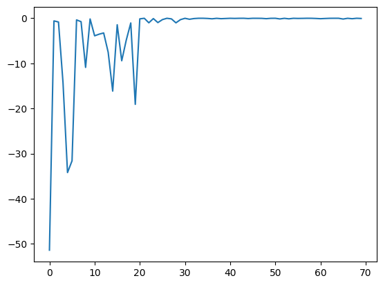
res is returned as an object of the history class (physbo.search.discrete.results.history).res.fx: The history of evaluated values of simulator (objective function).res.chosen_actions: The history of action IDs (parameters) when the simulator was evaluated.fbest, best_action= res.export_all_sequence_best_fx(): The history of best values and their action IDs (parameters) for all timings when the simulator was evaluated.res.total_num_search: Total number of simulator evaluations.
res.fx and best_fx should range up to res.total_num_search, respectively.[7]:
import matplotlib.pyplot as plt
%matplotlib inline
[8]:
plt.plot(res.fx[0:res.total_num_search])
[8]:
[<matplotlib.lines.Line2D at 0x129b7b5b0>]
[9]:
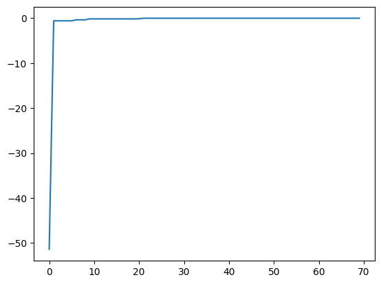
best_fx, best_action = res.export_all_sequence_best_fx()
plt.plot(best_fx)
[9]:
[<matplotlib.lines.Line2D at 0x129c6dc70>]
Serializing the results
The search results can be saved to an external file using the save method.
[10]:
res.save('search_result.npz')
[11]:
del res
Load the saved result file as follows:
[12]:
res = physbo.search.discrete.History()
res.load('search_result.npz')
Finally, the candidate with the best score can be displayed as follows. You can see that we have arrived at the correct solution \(x=-1\).
[13]:
print(X[int(best_action[-1])])
[-1.002]
Prediction
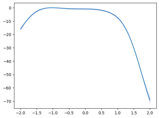
policy serves get_post_fmean and get_post_fcov methods for calculating mean value and variance of Gaussian process (post distribution).
[14]:
mean = policy.get_post_fmean(X)
var = policy.get_post_fcov(X)
std = np.sqrt(var)
xs = X[:,0]

ax = plt.subplot()
ax.plot(xs, mean)
ax.fill_between(xs, mean-std, mean+std, color="blue", alpha=.1)
[14]:
<matplotlib.collections.PolyCollection at 0x129d36520>
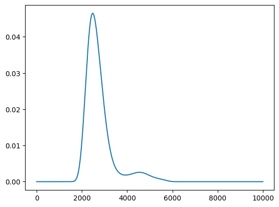
Acquisition function
policy serves get_score method for calculating acquisition function.
[15]:
scores = policy.get_score(mode="EI", xs=X)
plt.plot(scores)
[15]:
[<matplotlib.lines.Line2D at 0x129e19e50>]
Parallelization
PHYSBO can calculate acquisition functions for candidates in parallel by using MPI via mpi4py . To enable MPI parallelization, pass a MPI communicator such as MPI.COMM_WORLD to a keyword argument, comm of the constructor of the policy.
[16]:
# from mpi4py import MPI
# policy = physbo.search.discrete.policy(test_X=X, comm=MPI.COMM_WORLD)