This jupyter notebook file is available at ISSP Data Repository (v3.0.0 branch).
Search multiple candidates at once
This is a tutorial for evaluating two or more candidates at once in a single search step.
Prepare the search candidate data
As the previous tutorials, save the dataset file s5-210.csv and load dataset from this file as the following:
[1]:
import physbo

import numpy as np
import matplotlib.pyplot as plt
%matplotlib inline


def load_data():
    A =  np.asarray(np.loadtxt('s5-210.csv',skiprows=1, delimiter=',') )
    X = A[:,0:3]
    t  = -A[:,3]
    return X, t

X, t = load_data()
X = physbo.misc.centering(X)
Cythonized version of physbo is used
Definition of simulator
num_search_each_probe (described below) is set to 2 or more, action will be input as an array of action IDs.The definitions in the basic tutorial and simulator are the same, but keep in mind that t is a numpy.array, and when action is an array, self.t[action] will also be an array.
[2]:
class Simulator:
    def __init__( self ):
        _, self.t = load_data()

    def __call__( self, action ):
        return self.t[action]
Example of running the simulator
[3]:
sim = Simulator()
sim([1,12,123])
[3]:
array([-1.01487066, -1.22884748, -1.05572838])
Performing optimizations
[4]:
# set policy
policy = physbo.search.discrete.Policy(test_X=X)

# set seed
policy.set_seed( 0 )
num_search_each_probe allows you to specify the number of candidates to evaluate in each search step.
In the following example, the simulator will be evaluated 2 × 10 = 20 times by random search and 8 × 10 = 80 times by Bayesian optimization.
argument.
max_num_probes: Number of search steps.num_search_each_probe: Number of candidates to evaluate at each search step.
[5]:
res = policy.random_search(max_num_probes=2, num_search_each_probe=10, simulator=Simulator())

res = policy.bayes_search(max_num_probes=8, num_search_each_probe=10, simulator=Simulator(), score='EI',
                                                  interval=2, num_rand_basis=100)
0001-th multiple probe search (random)
current best f(x) = -0.980054 (best action = 4547)
list of simulation results
f(x)=-1.070602 (action = 15673)
f(x)=-1.009056 (action = 9559)
f(x)=-1.195844 (action = 16927)
f(x)=-0.980054 (action = 4547)
f(x)=-0.992820 (action = 2553)
f(x)=-1.146676 (action = 13144)
f(x)=-1.006255 (action = 10827)
f(x)=-0.999862 (action = 1995)
f(x)=-1.055445 (action = 10763)
f(x)=-1.100970 (action = 16450)


0002-th multiple probe search (random)
current best f(x) = -0.980054 (best action = 4547)
list of simulation results
f(x)=-1.208666 (action = 13085)
f(x)=-1.069404 (action = 15133)
f(x)=-1.031642 (action = 1706)
f(x)=-1.016702 (action = 2464)
f(x)=-1.172569 (action = 17812)
f(x)=-1.082219 (action = 16533)
f(x)=-1.025272 (action = 1336)
f(x)=-1.031761 (action = 10076)
f(x)=-0.984972 (action = 8876)
f(x)=-1.107730 (action = 15577)


Start the initial hyper parameter searching ...
Done

Start the hyper parameter learning ...
0 -th epoch marginal likelihood -22.83973847978999
50 -th epoch marginal likelihood -24.177617139908286
100 -th epoch marginal likelihood -24.831018285821855
150 -th epoch marginal likelihood -25.15416148652374
200 -th epoch marginal likelihood -25.33446562798866
250 -th epoch marginal likelihood -25.455155010625035
300 -th epoch marginal likelihood -25.550091453614577
350 -th epoch marginal likelihood -25.631301279338548
400 -th epoch marginal likelihood -25.702387457449046
450 -th epoch marginal likelihood -25.76434767734443
500 -th epoch marginal likelihood -25.817697844806304
Done

0003-th multiple probe search (EI)
current best f(x) = -0.963125 (best action = 7028)
list of simulation results
f(x)=-0.999831 (action = 8311)
f(x)=-0.971324 (action = 7695)
f(x)=-1.022353 (action = 11640)
f(x)=-2.231758 (action = 2989)
f(x)=-1.330630 (action = 14999)
f(x)=-1.490831 (action = 8998)
f(x)=-0.963461 (action = 8382)
f(x)=-1.006954 (action = 1144)
f(x)=-1.072227 (action = 8240)
f(x)=-0.963125 (action = 7028)


0004-th multiple probe search (EI)
current best f(x) = -0.963125 (best action = 7028)
list of simulation results
f(x)=-1.020075 (action = 2308)
f(x)=-1.013442 (action = 14800)
f(x)=-1.021923 (action = 2271)
f(x)=-1.008847 (action = 2272)
f(x)=-1.011485 (action = 2235)
f(x)=-1.124811 (action = 15021)
f(x)=-1.019125 (action = 2345)
f(x)=-1.034768 (action = 2344)
f(x)=-1.509526 (action = 15013)
f(x)=-1.007610 (action = 14763)


Start the initial hyper parameter searching ...
Done

Start the hyper parameter learning ...
0 -th epoch marginal likelihood 23.07362820544381
50 -th epoch marginal likelihood 9.71916785472228
100 -th epoch marginal likelihood 1.4617496079117842
150 -th epoch marginal likelihood -3.7988360129276657
200 -th epoch marginal likelihood -7.323789523166525
250 -th epoch marginal likelihood -9.785789330036444
300 -th epoch marginal likelihood -11.565934427597423
350 -th epoch marginal likelihood -12.890764162978346
400 -th epoch marginal likelihood -13.902281570598038
450 -th epoch marginal likelihood -14.69390233986634
500 -th epoch marginal likelihood -15.32925771239109
Done

0005-th multiple probe search (EI)
current best f(x) = -0.963125 (best action = 7028)
list of simulation results
f(x)=-1.065906 (action = 6464)
f(x)=-1.016857 (action = 9064)
f(x)=-1.052785 (action = 17091)
f(x)=-1.091519 (action = 14954)
f(x)=-0.984545 (action = 7141)
f(x)=-0.994764 (action = 3492)
f(x)=-0.986965 (action = 6497)
f(x)=-1.059148 (action = 5)
f(x)=-1.062454 (action = 16945)
f(x)=-1.076059 (action = 677)


0006-th multiple probe search (EI)
current best f(x) = -0.963125 (best action = 7028)
list of simulation results
f(x)=-0.990597 (action = 1590)
f(x)=-1.076706 (action = 13246)
f(x)=-1.145412 (action = 16280)
f(x)=-0.995306 (action = 11877)
f(x)=-1.023616 (action = 11106)
f(x)=-1.052131 (action = 11400)
f(x)=-0.991510 (action = 1627)
f(x)=-1.227426 (action = 6008)
f(x)=-0.965286 (action = 4587)
f(x)=-1.060802 (action = 13209)


Start the initial hyper parameter searching ...
Done

Start the hyper parameter learning ...
0 -th epoch marginal likelihood 473.65628141708936
50 -th epoch marginal likelihood 363.6169713454118
100 -th epoch marginal likelihood 280.4346034309078
150 -th epoch marginal likelihood 218.0054785862597
200 -th epoch marginal likelihood 170.65000562578464
250 -th epoch marginal likelihood 134.22268953329964
300 -th epoch marginal likelihood 105.78132811282697
350 -th epoch marginal likelihood 83.25038707552142
400 -th epoch marginal likelihood 65.1578863512562
450 -th epoch marginal likelihood 50.44852382153658
500 -th epoch marginal likelihood 38.355770381159886
Done

0007-th multiple probe search (EI)
current best f(x) = -0.960321 (best action = 8213)
list of simulation results
f(x)=-1.057612 (action = 14984)
f(x)=-0.990722 (action = 10878)
f(x)=-0.963464 (action = 8250)
f(x)=-1.043198 (action = 14947)
f(x)=-0.983485 (action = 10915)
f(x)=-0.968059 (action = 8287)
f(x)=-1.059552 (action = 14983)
f(x)=-0.999771 (action = 10841)
f(x)=-0.960321 (action = 8213)
f(x)=-0.977957 (action = 10952)


0008-th multiple probe search (EI)
current best f(x) = -0.960321 (best action = 8213)
list of simulation results
f(x)=-0.995292 (action = 703)
f(x)=-0.983678 (action = 8968)
f(x)=-0.997529 (action = 8967)
f(x)=-0.999770 (action = 666)
f(x)=-0.992400 (action = 740)
f(x)=-1.014959 (action = 4879)
f(x)=-0.977174 (action = 11967)
f(x)=-1.005922 (action = 629)
f(x)=-1.013689 (action = 592)
f(x)=-0.972775 (action = 8969)


Start the initial hyper parameter searching ...
Done

Start the hyper parameter learning ...
0 -th epoch marginal likelihood 70.33429991441193
50 -th epoch marginal likelihood 28.76449106005964
100 -th epoch marginal likelihood 0.48485195525671543
150 -th epoch marginal likelihood -18.236558043785863
200 -th epoch marginal likelihood -32.065352898632085
250 -th epoch marginal likelihood -42.76818194667307
300 -th epoch marginal likelihood -51.46052158149956
350 -th epoch marginal likelihood -56.687714339736516
400 -th epoch marginal likelihood -61.70347758865687
450 -th epoch marginal likelihood -65.19178853027769
500 -th epoch marginal likelihood -68.05551755259076
Done

0009-th multiple probe search (EI)
current best f(x) = -0.960321 (best action = 8213)
list of simulation results
f(x)=-1.055798 (action = 985)
f(x)=-0.997708 (action = 3033)
f(x)=-1.038770 (action = 1614)
f(x)=-1.031694 (action = 652)
f(x)=-1.033686 (action = 1207)
f(x)=-1.036349 (action = 763)
f(x)=-1.033301 (action = 1688)
f(x)=-1.045945 (action = 3133)
f(x)=-1.052235 (action = 947)
f(x)=-1.040833 (action = 430)


0010-th multiple probe search (EI)
current best f(x) = -0.960321 (best action = 8213)
list of simulation results
f(x)=-2.497328 (action = 17945)
f(x)=-0.990424 (action = 1480)
f(x)=-0.991675 (action = 5957)
f(x)=-0.990406 (action = 1517)
f(x)=-0.990488 (action = 1443)
f(x)=-1.094922 (action = 17908)
f(x)=-1.058552 (action = 3766)
f(x)=-1.053202 (action = 3803)
f(x)=-1.110345 (action = 15737)
f(x)=-0.990559 (action = 1554)
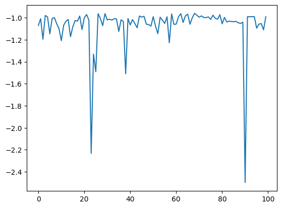
Checking results
[6]:
plt.plot(res.fx[0:res.total_num_search])
[6]:
[<matplotlib.lines.Line2D at 0x161abb310>]
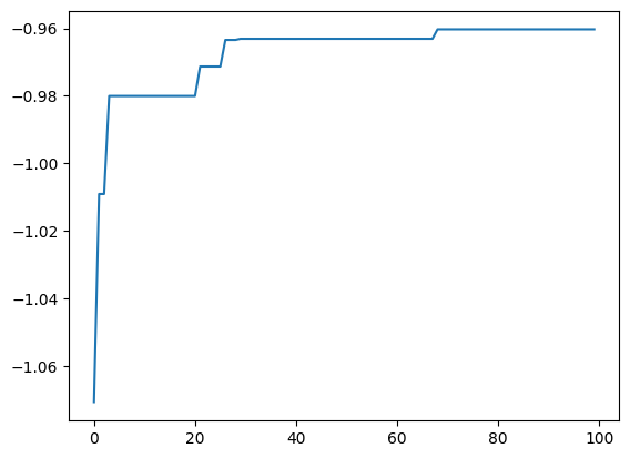
[7]:
best_fx, best_action = res.export_all_sequence_best_fx()
plt.plot(best_fx)
[7]:
[<matplotlib.lines.Line2D at 0x161bf6550>]
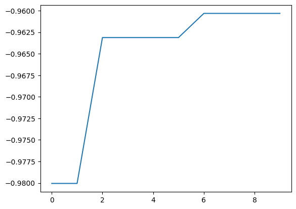
With res.export_sequence_best_fx(), you can get the best value obtained at each step and the history of the action.
The difference between res.export_all_sequence_best_fx() and res.export_all_sequence_best_fx() is that the information is not for each evaluation of the simulator, but for each search step. In this case, the total number of steps is 10, and the number of evaluations is 100.
[8]:
best_fx, best_action = res.export_sequence_best_fx()
plt.plot(best_fx)
[8]:
[<matplotlib.lines.Line2D at 0x161c68c70>]