This jupyter notebook file is available at ISSP Data Repository (v3.0.0 branch).

Optimization in Continuous Space

In the tutorials so far, we have been discretizing the feature space to perform Bayesian optimization. PHYSBO can also optimize while keeping quantities continuous.

As an algorithm for maximizing the acquisition function in continuous space, random search is implemented. Additionally, you can use ODAT-SE as an optimization library. This can be installed using pip.

python3 -m pip install odatse

Basic Usage

First, import the necessary modules.

import numpy as np
import physbo
import matplotlib.pyplot as plt

Cythonized version of physbo is used

The function simulator to be optimized, unlike the discrete version which received candidate point numbers action as input, in the continuous version directly receives coordinates x as input. x is an array of size \(N\times D\), where \(N\) is the number of data points to compute and \(D\) is the dimensionality of the features.

def simulator(x):
    return -np.sum(x**2, axis=1)

The lower and upper bounds of the feature space are specified by min_X and max_X respectively.

min_X = [-2.0, -2.0]
max_X = [2.0, 2.0]

The continuous space version of the Policy class is physbo.search.range.Policy. The constructor takes min_X and max_X as parameters. Also, similar to the discrete space version, you can enable parallel execution by passing mpi4py.MPI.Comm as comm. You can also set the random seed using the set_seed method.

seed = 31415
policy = physbo.search.range.Policy(min_X=min_X, max_X=max_X)
policy.set_seed(seed)

Once the Policy class is created, you can execute optimization following the same flow as the discrete space version. First, to create initial training data for learning the surrogate model, execute random_search.

policy.random_search(max_num_probes=10, simulator=simulator)

0001-th step: f(x) = -0.831185 (action=[0.58327442 0.70069668])
   current best f(x) = -0.831185 (best action=[0.58327442 0.70069668])

0002-th step: f(x) = -5.914186 (action=[1.88281594 1.53921746])
   current best f(x) = -0.831185 (best action=[0.58327442 0.70069668])

0003-th step: f(x) = -4.352756 (action=[1.63626337 1.29437187])
   current best f(x) = -0.831185 (best action=[0.58327442 0.70069668])

0004-th step: f(x) = -0.237057 (action=[-0.05316112  0.48397432])
   current best f(x) = -0.237057 (best action=[-0.05316112  0.48397432])

0005-th step: f(x) = -0.488353 (action=[ 0.57404985 -0.39852174])
   current best f(x) = -0.237057 (best action=[-0.05316112  0.48397432])

0006-th step: f(x) = -2.441356 (action=[1.50087645 0.43442582])
   current best f(x) = -0.237057 (best action=[-0.05316112  0.48397432])

0007-th step: f(x) = -3.440784 (action=[-1.57320004 -0.98276443])
   current best f(x) = -0.237057 (best action=[-0.05316112  0.48397432])

0008-th step: f(x) = -3.452632 (action=[-1.85812001  0.00465691])
   current best f(x) = -0.237057 (best action=[-0.05316112  0.48397432])

0009-th step: f(x) = -0.764532 (action=[ 0.46977882 -0.73745485])
   current best f(x) = -0.237057 (best action=[-0.05316112  0.48397432])

0010-th step: f(x) = -1.850471 (action=[-0.63939092 -1.20068727])
   current best f(x) = -0.237057 (best action=[-0.05316112  0.48397432])

<physbo.search.range._history.History at 0x103cf6400>

Next, execute Bayesian optimization with bayes_search.

res = policy.bayes_search(max_num_probes=10, simulator=simulator, score="EI")

Start the initial hyper parameter searching ...
Done

Start the hyper parameter learning ...
0 -th epoch marginal likelihood 14.586042968393606
50 -th epoch marginal likelihood 14.234874815492592
100 -th epoch marginal likelihood 14.063504009485214
150 -th epoch marginal likelihood 13.916750623078872
200 -th epoch marginal likelihood 13.772691286779512
250 -th epoch marginal likelihood 13.633003306706115
300 -th epoch marginal likelihood 13.49920085405347
350 -th epoch marginal likelihood 13.371932369305052
400 -th epoch marginal likelihood 13.251396114620242
450 -th epoch marginal likelihood 13.13755169992651
500 -th epoch marginal likelihood 13.03022856247339
Done

0011-th step: f(x) = -5.026362 (action=[-1.03592362  1.98827161])
   current best f(x) = -0.237057 (best action=[-0.05316112  0.48397432])

0012-th step: f(x) = -0.028634 (action=[0.1327553  0.10492853])
   current best f(x) = -0.028634 (best action=[0.1327553  0.10492853])

0013-th step: f(x) = -0.013414 (action=[0.07031902 0.09202588])
   current best f(x) = -0.013414 (best action=[0.07031902 0.09202588])

0014-th step: f(x) = -0.057856 (action=[0.23418776 0.05488579])
   current best f(x) = -0.013414 (best action=[0.07031902 0.09202588])

0015-th step: f(x) = -0.012249 (action=[ 0.110677   -0.00028234])
   current best f(x) = -0.012249 (best action=[ 0.110677   -0.00028234])

0016-th step: f(x) = -0.015602 (action=[0.12295699 0.02198239])
   current best f(x) = -0.012249 (best action=[ 0.110677   -0.00028234])

0017-th step: f(x) = -0.026756 (action=[0.11124983 0.11991566])
   current best f(x) = -0.012249 (best action=[ 0.110677   -0.00028234])

0018-th step: f(x) = -0.025519 (action=[0.13646757 0.08304057])
   current best f(x) = -0.012249 (best action=[ 0.110677   -0.00028234])

0019-th step: f(x) = -0.005797 (action=[0.07576489 0.00754463])
   current best f(x) = -0.005797 (best action=[0.07576489 0.00754463])

0020-th step: f(x) = -0.032290 (action=[0.09645697 0.15161167])
   current best f(x) = -0.005797 (best action=[0.07576489 0.00754463])

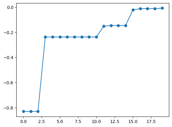
The return value res of the bayes_search function contains the process of Bayesian optimization. Using the export_sequence_best_fx method, you can obtain the optimization results at each step.

best_fx, best_X = res.export_sequence_best_fx()

plt.plot(best_fx, "o-")

[<matplotlib.lines.Line2D at 0x1350051f0>]

Acquisition Function Optimization Algorithm

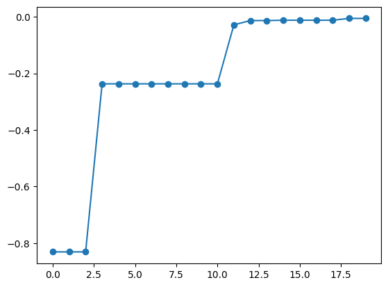
For acquisition function optimization, random search is performed by default. This means that nsamples = 1000 candidate points are randomly selected, and the point with the largest acquisition function among them is chosen. To change the value of nsamples, use physbo.search.optimizer.random.Optimizer. For example, if you want to set nsamples = 100, create random_optimizer as follows and pass it to the optimizer keyword of the bayes_search function.

random_optimizer = physbo.search.optimize.random.Optimizer(min_X=min_X, max_X=max_X, nsamples=100)

policy = physbo.search.range.Policy(min_X=min_X, max_X=max_X)
policy.set_seed(seed)
policy.random_search(max_num_probes=10, simulator=simulator)

res = policy.bayes_search(max_num_probes=10, simulator=simulator, score="EI", optimizer=random_optimizer)

best_fx, best_X = res.export_sequence_best_fx()

plt.plot(best_fx, "o-")

0001-th step: f(x) = -0.831185 (action=[0.58327442 0.70069668])
   current best f(x) = -0.831185 (best action=[0.58327442 0.70069668])

0002-th step: f(x) = -5.914186 (action=[1.88281594 1.53921746])
   current best f(x) = -0.831185 (best action=[0.58327442 0.70069668])

0003-th step: f(x) = -4.352756 (action=[1.63626337 1.29437187])
   current best f(x) = -0.831185 (best action=[0.58327442 0.70069668])

0004-th step: f(x) = -0.237057 (action=[-0.05316112  0.48397432])
   current best f(x) = -0.237057 (best action=[-0.05316112  0.48397432])

0005-th step: f(x) = -0.488353 (action=[ 0.57404985 -0.39852174])
   current best f(x) = -0.237057 (best action=[-0.05316112  0.48397432])

0006-th step: f(x) = -2.441356 (action=[1.50087645 0.43442582])
   current best f(x) = -0.237057 (best action=[-0.05316112  0.48397432])

0007-th step: f(x) = -3.440784 (action=[-1.57320004 -0.98276443])
   current best f(x) = -0.237057 (best action=[-0.05316112  0.48397432])

0008-th step: f(x) = -3.452632 (action=[-1.85812001  0.00465691])
   current best f(x) = -0.237057 (best action=[-0.05316112  0.48397432])

0009-th step: f(x) = -0.764532 (action=[ 0.46977882 -0.73745485])
   current best f(x) = -0.237057 (best action=[-0.05316112  0.48397432])

0010-th step: f(x) = -1.850471 (action=[-0.63939092 -1.20068727])
   current best f(x) = -0.237057 (best action=[-0.05316112  0.48397432])

Start the initial hyper parameter searching ...
Done

Start the hyper parameter learning ...
0 -th epoch marginal likelihood 14.586042968393606
50 -th epoch marginal likelihood 14.234874815492592
100 -th epoch marginal likelihood 14.063504009485214
150 -th epoch marginal likelihood 13.916750623078872
200 -th epoch marginal likelihood 13.772691286779512
250 -th epoch marginal likelihood 13.633003306706115
300 -th epoch marginal likelihood 13.49920085405347
350 -th epoch marginal likelihood 13.371932369305052
400 -th epoch marginal likelihood 13.251396114620242
450 -th epoch marginal likelihood 13.13755169992651
500 -th epoch marginal likelihood 13.03022856247339
Done

0011-th step: f(x) = -3.969688 (action=[-0.55371092  1.91392061])
   current best f(x) = -0.237057 (best action=[-0.05316112  0.48397432])

0012-th step: f(x) = -0.048301 (action=[ 0.09981879 -0.19579904])
   current best f(x) = -0.048301 (best action=[ 0.09981879 -0.19579904])

0013-th step: f(x) = -0.026065 (action=[0.00582793 0.16134044])
   current best f(x) = -0.026065 (best action=[0.00582793 0.16134044])

0014-th step: f(x) = -0.029637 (action=[-0.03315978  0.16893146])
   current best f(x) = -0.026065 (best action=[0.00582793 0.16134044])

0015-th step: f(x) = -6.287502 (action=[ 1.84812961 -1.69467382])
   current best f(x) = -0.026065 (best action=[0.00582793 0.16134044])

0016-th step: f(x) = -0.007927 (action=[ 0.06895685 -0.05632176])
   current best f(x) = -0.007927 (best action=[ 0.06895685 -0.05632176])

0017-th step: f(x) = -0.011240 (action=[0.10157691 0.03036993])
   current best f(x) = -0.007927 (best action=[ 0.06895685 -0.05632176])

0018-th step: f(x) = -0.060419 (action=[ 0.1940892  -0.15082425])
   current best f(x) = -0.007927 (best action=[ 0.06895685 -0.05632176])

0019-th step: f(x) = -0.016852 (action=[-0.12738362  0.02501082])
   current best f(x) = -0.007927 (best action=[ 0.06895685 -0.05632176])

0020-th step: f(x) = -0.093609 (action=[0.12668816 0.27849452])
   current best f(x) = -0.007927 (best action=[ 0.06895685 -0.05632176])

[<matplotlib.lines.Line2D at 0x1350f0610>]

Using optimizers other than physbo.search.optimizer.random.Optimizer, you can utilize maximization algorithms other than random search. PHYSBO provides an optimizer using ODAT-SE: physbo.search.optimize.odatse.Optimizer. This library can solve optimization problems using five algorithms:

• “exchange”: Replica exchange Monte Carlo method

• “pamc”: Population annealing Monte Carlo method

• “minsearch”: Nelder-Mead method

• “mapper”: Grid search

• “bayes”: Bayesian optimization

The algorithms and hyperparameters of ODAT-SE are specified using a dictionary equivalent to the [algorithm] section of the ODAT-SE input file.

The physbo.search.optimize.odatse.default_alg_dict function creates a template for this dictionary, so modify the parameters as needed.

import physbo.search.optimize.odatse
odatse_alg_dict = physbo.search.optimize.odatse.default_alg_dict(min_X=min_X, max_X=max_X, algorithm_name="exchange")

# show the default parameters for the exchange algorithm
odatse_alg_dict

{'name': 'exchange',
 'seed': 12345,
 'param': {'min_list': array([-2., -2.]),
  'max_list': array([2., 2.]),
  'step_list': array([0.04, 0.04])},
 'exchange': {'numsteps': 1000,
  'numsteps_exchange': 10,
  'Tmin': 0.1,
  'Tmax': 10.0,
  'Tlogspace': True,
  'nreplica_per_proc': 10}}

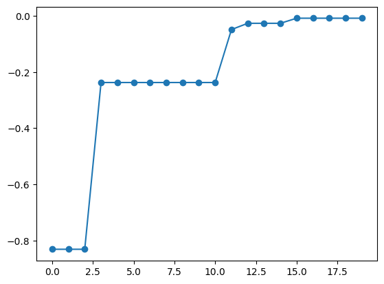
Pass odatse_alg_dict to physbo.search.optimize.odatse.Optimizer to create the optimizer odatse_optimizer. By passing this to the optimizer keyword of the bayes_search function, similar to random_optimizer, you can perform optimization using ODAT-SE.

odatse_optimizer = physbo.search.optimize.odatse.Optimizer(alg_dict=odatse_alg_dict)

policy = physbo.search.range.Policy(min_X=min_X, max_X=max_X)
policy.set_seed(seed)
policy.random_search(max_num_probes=10, simulator=simulator)

res = policy.bayes_search(max_num_probes=10, simulator=simulator, optimizer=odatse_optimizer, score="EI")

best_fx, best_X = res.export_sequence_best_fx()

plt.plot(best_fx, "o-")

[<matplotlib.lines.Line2D at 0x136bf8f10>]