この jupyter notebook ファイルは ISSP Data Repository (v3.0.0 branch) から入手できます。
多目的最適化
\(y \prec y^{'}\Longleftrightarrow \forall \ i \le p, y_i \le y^{'}_i \land \exists \ j \le p, y_j < y^{'}_j\)
PHYSBOでは、パレート解を効率的に求めるためのベイズ最適化手法を実装しています。
[1]:
import numpy as np
import matplotlib.pyplot as plt
import physbo
%matplotlib inline
Cythonized version of physbo is used
テスト関数
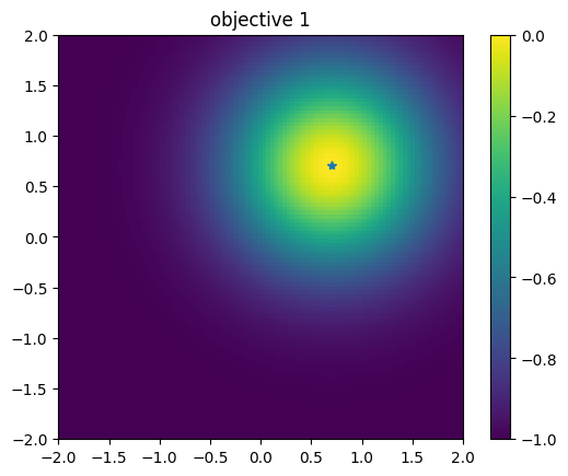
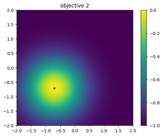
\(y_1\) と \(y_2\) はそれぞれ \(x_1 = x_2 = \cdots x_N = 1/\sqrt{N}\) と \(x_1 = x_2 = \cdots x_N = -1/\sqrt{N}\) に最小値があり、その値はともに0です。また、上界は1 です。
PHYSBO は最大化問題を仮定するため、-1を掛けたものをあらためて目的関数とします。
参考文献
Van Veldhuizen, David A. Multiobjective evolutionary algorithms: classifications, analyses, and new innovations. No. AFIT/DS/ENG/99-01. AIR FORCE INST OF TECH WRIGHT-PATTERSONAFB OH SCHOOL OF ENGINEERING, 1999.
[2]:
def vlmop2_minus(x):
    n = x.shape[1]
    y1 = 1 - np.exp(-1 * np.sum((x - 1/np.sqrt(n)) ** 2, axis = 1))
    y2 = 1 - np.exp(-1 * np.sum((x + 1/np.sqrt(n)) ** 2, axis = 1))

    return np.c_[-y1, -y2]
探索候補データの準備
入力空間 \(\vec{x}\) は 2次元とし、[-2, 2] × [-2, 2] の上で候補点をグリッド状に生成します。
[3]:
import itertools
a = np.linspace(-2,2,101)
test_X = np.array(list(itertools.product(a, a)))
[4]:
test_X
[4]:
array([[-2.  , -2.  ],
       [-2.  , -1.96],
       [-2.  , -1.92],
       ...,
       [ 2.  ,  1.92],
       [ 2.  ,  1.96],
       [ 2.  ,  2.  ]])
[5]:
test_X.shape
[5]:
(10201, 2)
simulator の定義
[6]:
class Simulator(object):
    def __init__(self, X):
        self.t = vlmop2_minus(X)

    def __call__( self, action):
        return self.t[action]
[7]:
simu = Simulator(test_X)
関数のプロット
1つ目の目的関数
[8]:
plt.figure()
plt.imshow(simu.t[:,0].reshape((101,101)), vmin=-1.0, vmax=0.0, origin="lower", extent=[-2.0, 2.0, -2.0, 2.0])
plt.title("objective 1")
plt.colorbar()
plt.plot([1.0/np.sqrt(2.0)], [1.0/np.sqrt(2.0)], '*')
plt.show()
2つ目の目的関数
[9]:
# plot objective 2
plt.figure()
plt.imshow(simu.t[:,1].reshape((101,101)), vmin=-1.0, vmax=0.0, origin="lower", extent=[-2.0, 2.0, -2.0, 2.0])
plt.title("objective 2")
plt.colorbar()
plt.plot([-1.0/np.sqrt(2.0)], [-1.0/np.sqrt(2.0)], '*')
plt.show()
最適化の実行
Policy のセット
physbo.search.discrete_multi.Policy を利用します。num_objectives に目的関数の数を指定してください。[10]:
policy = physbo.search.discrete_multi.Policy(test_X=test_X, num_objectives=2)
policy.set_seed(0)
physbo.search.discrete.policy (目的関数が1つの場合)と同じく、random_search または bayes_search メソッドを呼ぶことで最適化を行います。discrete.policy とおおよそ共通しています。ランダムサーチ
[11]:
policy = physbo.search.discrete_multi.Policy(test_X=test_X, num_objectives=2)
policy.set_seed(0)

res_random = policy.random_search(max_num_probes=50, simulator=simu)
0001-th step: f(x) = [-0.99973003 -0.62334035] (action = 836)
   Pareto set updated.
   the number of Pareto frontiers = 1

0002-th step: f(x) = [-0.99789981 -0.99866427] (action = 9404)
   Pareto set updated.
   the number of Pareto frontiers = 2

0003-th step: f(x) = [-0.99090897 -0.46609239] (action = 4664)
   Pareto set updated.
   the number of Pareto frontiers = 1

0004-th step: f(x) = [-0.92633083 -0.29208351] (action = 4780)
   Pareto set updated.
   the number of Pareto frontiers = 1

0005-th step: f(x) = [-0.67969326 -0.99981691] (action = 9566)
   Pareto set updated.
   the number of Pareto frontiers = 2

0006-th step: f(x) = [-0.45601619 -0.99848443] (action = 8852)
   Pareto set updated.
   the number of Pareto frontiers = 2

0007-th step: f(x) = [-0.92670204 -0.71508873] (action = 6088)
0008-th step: f(x) = [-0.58233995 -0.99952931] (action = 7060)
0009-th step: f(x) = [-0.99848229 -0.96780195] (action = 473)
0010-th step: f(x) = [-0.80479332 -0.99994946] (action = 7573)
0011-th step: f(x) = [-0.99700074 -0.99847873] (action = 1406)
0012-th step: f(x) = [-0.9992592  -0.93891121] (action = 6061)
0013-th step: f(x) = [-0.19963873 -0.93357674] (action = 5722)
   Pareto set updated.
   the number of Pareto frontiers = 2

0014-th step: f(x) = [-0.98046765 -0.99294428] (action = 2309)
0015-th step: f(x) = [-0.99602549 -0.98620358] (action = 7989)
0016-th step: f(x) = [-0.99957128 -0.9973798 ] (action = 8484)
0017-th step: f(x) = [-0.52191048 -0.72845916] (action = 5405)
   Pareto set updated.
   the number of Pareto frontiers = 3

0018-th step: f(x) = [-0.99916441 -0.40869572] (action = 2742)
0019-th step: f(x) = [-0.99480122 -0.7565076 ] (action = 1266)
0020-th step: f(x) = [-0.63329589 -0.63329589] (action = 5200)
   Pareto set updated.
   the number of Pareto frontiers = 4

0021-th step: f(x) = [-0.95437918 -0.80142908] (action = 2487)
0022-th step: f(x) = [-0.99899466 -0.96646532] (action = 269)
0023-th step: f(x) = [-0.19473522 -0.99445365] (action = 8044)
   Pareto set updated.
   the number of Pareto frontiers = 5

0024-th step: f(x) = [-0.99969529 -0.52395588] (action = 2135)
0025-th step: f(x) = [-0.59106078 -0.79258035] (action = 6206)
0026-th step: f(x) = [-0.78231041 -0.99997141] (action = 9079)
0027-th step: f(x) = [-0.99955573 -0.99930147] (action = 396)
0028-th step: f(x) = [-0.99825097 -0.99875436] (action = 9403)
0029-th step: f(x) = [-0.65387719 -0.99938669] (action = 9456)
0030-th step: f(x) = [-0.26132949 -0.87913689] (action = 5816)
   Pareto set updated.
   the number of Pareto frontiers = 6

0031-th step: f(x) = [-0.74523952 -0.7724917 ] (action = 6301)
0032-th step: f(x) = [-0.33644513 -0.97772424] (action = 5530)
0033-th step: f(x) = [-0.99777557 -0.93373833] (action = 6470)
0034-th step: f(x) = [-0.9725524 -0.6296562] (action = 2277)
0035-th step: f(x) = [-0.99924826 -0.84674905] (action = 353)
0036-th step: f(x) = [-0.99743705 -0.17848438] (action = 2549)
   Pareto set updated.
   the number of Pareto frontiers = 7

0037-th step: f(x) = [-0.99994916 -0.78013199] (action = 326)
0038-th step: f(x) = [-0.99887174 -0.86936149] (action = 5458)
0039-th step: f(x) = [-0.99362699 -0.99769786] (action = 9309)
0040-th step: f(x) = [-0.84889217 -0.99973225] (action = 10156)
0041-th step: f(x) = [-0.95713719 -0.09067194] (action = 4073)
   Pareto set updated.
   the number of Pareto frontiers = 7

0042-th step: f(x) = [-0.17190645 -0.91382463] (action = 6120)
   Pareto set updated.
   the number of Pareto frontiers = 6

0043-th step: f(x) = [-0.98406208 -0.94467587] (action = 7289)
0044-th step: f(x) = [-0.93974303 -0.92444262] (action = 2698)
0045-th step: f(x) = [-0.98414342 -0.84762781] (action = 1780)
0046-th step: f(x) = [-0.99699986 -0.98166426] (action = 7684)
0047-th step: f(x) = [-0.3868143  -0.99930896] (action = 8060)
0048-th step: f(x) = [-0.97964062 -0.65554315] (action = 2075)
0049-th step: f(x) = [-0.99907307 -0.73466786] (action = 4450)
0050-th step: f(x) = [-0.99720717 -0.85352507] (action = 865)
disp_pareto_set=True と指定します。[12]:
policy = physbo.search.discrete_multi.Policy(test_X=test_X, num_objectives=2)
policy.set_seed(0)
res_random = policy.random_search(max_num_probes=50, simulator=simu, disp_pareto_set=True)
0001-th step: f(x) = [-0.99973003 -0.62334035] (action = 836)
   Pareto set updated.
   current Pareto set = [[-0.99973003 -0.62334035]] (steps = [1])

0002-th step: f(x) = [-0.99789981 -0.99866427] (action = 9404)
   Pareto set updated.
   current Pareto set = [[-0.99973003 -0.62334035]
 [-0.99789981 -0.99866427]] (steps = [1 2])

0003-th step: f(x) = [-0.99090897 -0.46609239] (action = 4664)
   Pareto set updated.
   current Pareto set = [[-0.99090897 -0.46609239]] (steps = [3])

0004-th step: f(x) = [-0.92633083 -0.29208351] (action = 4780)
   Pareto set updated.
   current Pareto set = [[-0.92633083 -0.29208351]] (steps = [4])

0005-th step: f(x) = [-0.67969326 -0.99981691] (action = 9566)
   Pareto set updated.
   current Pareto set = [[-0.92633083 -0.29208351]
 [-0.67969326 -0.99981691]] (steps = [4 5])

0006-th step: f(x) = [-0.45601619 -0.99848443] (action = 8852)
   Pareto set updated.
   current Pareto set = [[-0.92633083 -0.29208351]
 [-0.45601619 -0.99848443]] (steps = [4 6])

0007-th step: f(x) = [-0.92670204 -0.71508873] (action = 6088)
0008-th step: f(x) = [-0.58233995 -0.99952931] (action = 7060)
0009-th step: f(x) = [-0.99848229 -0.96780195] (action = 473)
0010-th step: f(x) = [-0.80479332 -0.99994946] (action = 7573)
0011-th step: f(x) = [-0.99700074 -0.99847873] (action = 1406)
0012-th step: f(x) = [-0.9992592  -0.93891121] (action = 6061)
0013-th step: f(x) = [-0.19963873 -0.93357674] (action = 5722)
   Pareto set updated.
   current Pareto set = [[-0.92633083 -0.29208351]
 [-0.19963873 -0.93357674]] (steps = [ 4 13])

0014-th step: f(x) = [-0.98046765 -0.99294428] (action = 2309)
0015-th step: f(x) = [-0.99602549 -0.98620358] (action = 7989)
0016-th step: f(x) = [-0.99957128 -0.9973798 ] (action = 8484)
0017-th step: f(x) = [-0.52191048 -0.72845916] (action = 5405)
   Pareto set updated.
   current Pareto set = [[-0.92633083 -0.29208351]
 [-0.52191048 -0.72845916]
 [-0.19963873 -0.93357674]] (steps = [ 4 17 13])

0018-th step: f(x) = [-0.99916441 -0.40869572] (action = 2742)
0019-th step: f(x) = [-0.99480122 -0.7565076 ] (action = 1266)
0020-th step: f(x) = [-0.63329589 -0.63329589] (action = 5200)
   Pareto set updated.
   current Pareto set = [[-0.92633083 -0.29208351]
 [-0.63329589 -0.63329589]
 [-0.52191048 -0.72845916]
 [-0.19963873 -0.93357674]] (steps = [ 4 20 17 13])

0021-th step: f(x) = [-0.95437918 -0.80142908] (action = 2487)
0022-th step: f(x) = [-0.99899466 -0.96646532] (action = 269)
0023-th step: f(x) = [-0.19473522 -0.99445365] (action = 8044)
   Pareto set updated.
   current Pareto set = [[-0.92633083 -0.29208351]
 [-0.63329589 -0.63329589]
 [-0.52191048 -0.72845916]
 [-0.19963873 -0.93357674]
 [-0.19473522 -0.99445365]] (steps = [ 4 20 17 13 23])

0024-th step: f(x) = [-0.99969529 -0.52395588] (action = 2135)
0025-th step: f(x) = [-0.59106078 -0.79258035] (action = 6206)
0026-th step: f(x) = [-0.78231041 -0.99997141] (action = 9079)
0027-th step: f(x) = [-0.99955573 -0.99930147] (action = 396)
0028-th step: f(x) = [-0.99825097 -0.99875436] (action = 9403)
0029-th step: f(x) = [-0.65387719 -0.99938669] (action = 9456)
0030-th step: f(x) = [-0.26132949 -0.87913689] (action = 5816)
   Pareto set updated.
   current Pareto set = [[-0.92633083 -0.29208351]
 [-0.63329589 -0.63329589]
 [-0.52191048 -0.72845916]
 [-0.26132949 -0.87913689]
 [-0.19963873 -0.93357674]
 [-0.19473522 -0.99445365]] (steps = [ 4 20 17 30 13 23])

0031-th step: f(x) = [-0.74523952 -0.7724917 ] (action = 6301)
0032-th step: f(x) = [-0.33644513 -0.97772424] (action = 5530)
0033-th step: f(x) = [-0.99777557 -0.93373833] (action = 6470)
0034-th step: f(x) = [-0.9725524 -0.6296562] (action = 2277)
0035-th step: f(x) = [-0.99924826 -0.84674905] (action = 353)
0036-th step: f(x) = [-0.99743705 -0.17848438] (action = 2549)
   Pareto set updated.
   current Pareto set = [[-0.99743705 -0.17848438]
 [-0.92633083 -0.29208351]
 [-0.63329589 -0.63329589]
 [-0.52191048 -0.72845916]
 [-0.26132949 -0.87913689]
 [-0.19963873 -0.93357674]
 [-0.19473522 -0.99445365]] (steps = [36  4 20 17 30 13 23])

0037-th step: f(x) = [-0.99994916 -0.78013199] (action = 326)
0038-th step: f(x) = [-0.99887174 -0.86936149] (action = 5458)
0039-th step: f(x) = [-0.99362699 -0.99769786] (action = 9309)
0040-th step: f(x) = [-0.84889217 -0.99973225] (action = 10156)
0041-th step: f(x) = [-0.95713719 -0.09067194] (action = 4073)
   Pareto set updated.
   current Pareto set = [[-0.95713719 -0.09067194]
 [-0.92633083 -0.29208351]
 [-0.63329589 -0.63329589]
 [-0.52191048 -0.72845916]
 [-0.26132949 -0.87913689]
 [-0.19963873 -0.93357674]
 [-0.19473522 -0.99445365]] (steps = [41  4 20 17 30 13 23])

0042-th step: f(x) = [-0.17190645 -0.91382463] (action = 6120)
   Pareto set updated.
   current Pareto set = [[-0.95713719 -0.09067194]
 [-0.92633083 -0.29208351]
 [-0.63329589 -0.63329589]
 [-0.52191048 -0.72845916]
 [-0.26132949 -0.87913689]
 [-0.17190645 -0.91382463]] (steps = [41  4 20 17 30 42])

0043-th step: f(x) = [-0.98406208 -0.94467587] (action = 7289)
0044-th step: f(x) = [-0.93974303 -0.92444262] (action = 2698)
0045-th step: f(x) = [-0.98414342 -0.84762781] (action = 1780)
0046-th step: f(x) = [-0.99699986 -0.98166426] (action = 7684)
0047-th step: f(x) = [-0.3868143  -0.99930896] (action = 8060)
0048-th step: f(x) = [-0.97964062 -0.65554315] (action = 2075)
0049-th step: f(x) = [-0.99907307 -0.73466786] (action = 4450)
0050-th step: f(x) = [-0.99720717 -0.85352507] (action = 865)
結果の確認
#### 評価値の履歴
[ ]:
res_random.fx[0:res_random.num_runs]
パレート解の取得
[14]:
front, front_num = res_random.export_pareto_front()
front, front_num
[14]:
(array([[-0.95713719, -0.09067194],
        [-0.92633083, -0.29208351],
        [-0.63329589, -0.63329589],
        [-0.52191048, -0.72845916],
        [-0.26132949, -0.87913689],
        [-0.17190645, -0.91382463]]),
 array([40,  3, 19, 16, 29, 41]))
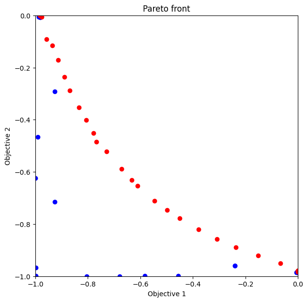
解(評価値)のプロット
これ以降、図示する空間が \(y = (y_1, y_2)\) であり \(x = (x_1, x_2)\) ではないことにあらためて注意してください。
赤のプロットがパレート解です。
[15]:
def plot_pareto_front(res):
    front, front_num = res.export_pareto_front()
    dominated = [i for i in range(res.num_runs) if i not in front_num]
    points = res.fx[dominated, :]

    plt.figure(figsize=(7, 7))
    plt.scatter(res.fx[dominated,0], res.fx[dominated,1], c = "blue")
    plt.scatter(front[:, 0], front[:, 1], c = "red")
    plt.title('Pareto front')
    plt.xlabel('Objective 1')
    plt.ylabel('Objective 2')
    plt.xlim([-1.0,0.0])
    plt.ylim([-1.0,0.0])
[16]:
plot_pareto_front(res_random)
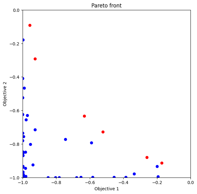
劣解領域 (dominated region) の体積を計算
res_random.pareto.volume_in_dominance(ref_min, ref_max) は、 ref_min, ref_max で指定された矩形(hyper-rectangle) 中の劣解領域体積を計算します。
[17]:
res_random.pareto.volume_in_dominance([-1,-1],[0,0])
[17]:
0.2376881844865093
ベイズ最適化
多目的の場合の bayes_search では、score には以下のいずれかを指定します。
HVPI (HyperVolume-based Probability of Improvement)
EHVI (Expected Hyper-Volume Improvement)
TS (Thompson Sampling)
以下、score を変えてそれぞれ 50回 (ランダムサーチ10回 + ベイズ最適化 40回) 評価を行います。
HVPI (HyperVolume-based Probability of Improvement)
多次元の目的関数空間における非劣解領域 (non-dominated region) の改善確率を score として求めます。
参考文献
Couckuyt, Ivo, Dirk Deschrijver, and Tom Dhaene. 「Fast calculation of multiobjective probability of improvement and expected improvement criteria for Pareto optimization.」 Journal of Global Optimization 60.3 (2014): 575-594.
[ ]:
policy = physbo.search.discrete_multi.Policy(test_X=test_X, num_objectives=2)
policy.set_seed(0)

policy.random_search(max_num_probes=10, simulator=simu)
res_HVPI = policy.bayes_search(max_num_probes=40, simulator=simu, score='HVPI', interval=10)
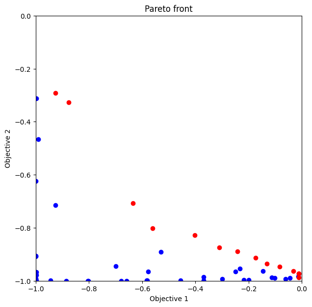
パレート解のプロット
ランダムサンプリングと比較して、パレート解が多く求まっていることが分かります。
[19]:
plot_pareto_front(res_HVPI)
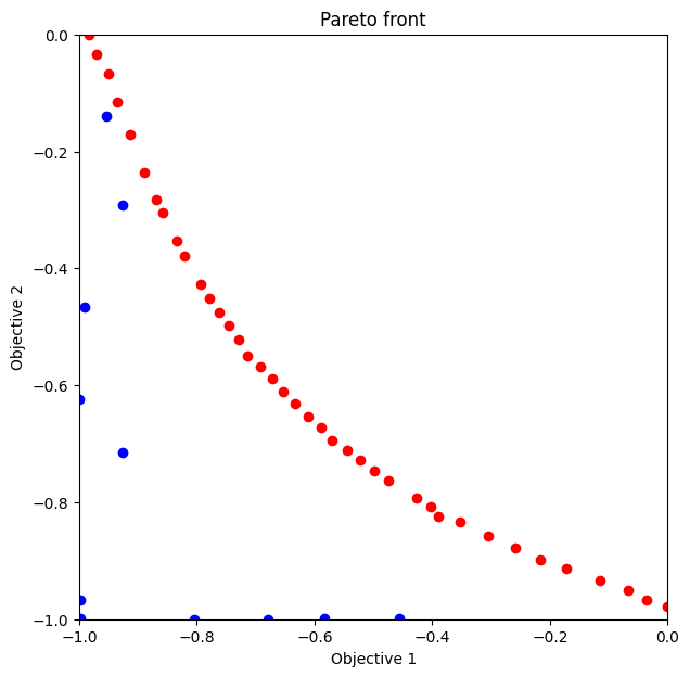
劣解領域体積
[20]:
res_HVPI.pareto.volume_in_dominance([-1,-1],[0,0])
[20]:
0.32877907991633726
EHVI (Expected Hyper-Volume Improvement)
多次元の目的関数空間における非劣解領域 (non-dominated region) の改善期待値を score として求めます。
参考文献
Couckuyt, Ivo, Dirk Deschrijver, and Tom Dhaene. 「Fast calculation of multiobjective probability of improvement and expected improvement criteria for Pareto optimization.」 Journal of Global Optimization 60.3 (2014): 575-594.
[ ]:
policy = physbo.search.discrete_multi.Policy(test_X=test_X, num_objectives=2)
policy.set_seed(0)

policy.random_search(max_num_probes=10, simulator=simu)
res_EHVI = policy.bayes_search(max_num_probes=40, simulator=simu, score='EHVI', interval=10)
パレート解のプロット
[22]:
plot_pareto_front(res_EHVI)
劣解領域体積
[23]:
res_EHVI.pareto.volume_in_dominance([-1,-1],[0,0])
[23]:
0.3200467412741881
TS (Thompson Sampling)
参考文献
Yahyaa, Saba Q., and Bernard Manderick. 「Thompson sampling for multi-objective multi-armed bandits problem.」 Proc. Eur. Symp. Artif. Neural Netw., Comput. Intell. Mach. Learn.. 2015.
[ ]:
policy = physbo.search.discrete_multi.Policy(test_X=test_X, num_objectives=2)
policy.set_seed(0)

policy.random_search(max_num_probes=10, simulator=simu)
res_TS = policy.bayes_search(max_num_probes=40, simulator=simu, score='TS', interval=10, num_rand_basis=5000)
パレート解のプロット
[25]:
plot_pareto_front(res_TS)
劣解領域体積
[26]:
res_TS.pareto.volume_in_dominance([-1,-1],[0,0])
[26]:
0.23103794208330097
付録:全探索
random_search で max_num_probes に全データ数 (N = test_X.shape[0]) を渡すと手軽に全探索できます。[ ]:
test_X_sparse = np.array(list(itertools.product(np.linspace(-2, 2, 21), repeat=2)))
simu_sparse = Simulator(test_X_sparse)

policy = physbo.search.discrete_multi.Policy(test_X=test_X_sparse, num_objectives=2)
policy.set_seed(0)

N = test_X_sparse.shape[0]
res_all = policy.random_search(max_num_probes=N, simulator=simu_sparse)
[28]:
plot_pareto_front(res_all)
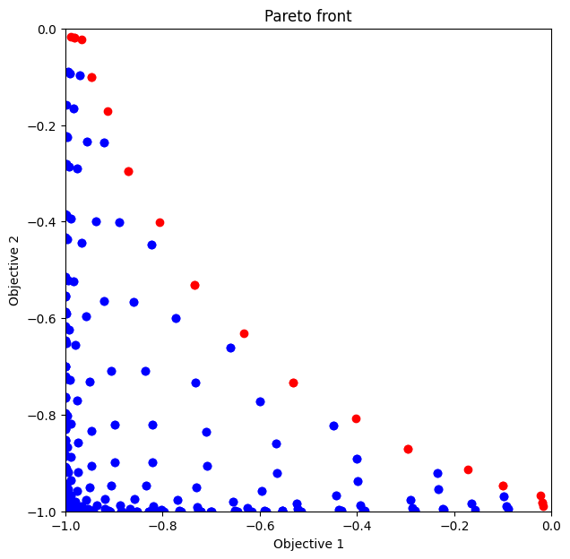
[29]:
res_all.pareto.volume_in_dominance([-1,-1],[0,0])
[29]:
0.30051687493437484