この jupyter notebook ファイルは ISSP Data Repository (v3.0.0 branch) から入手できます。
複数候補を一度に探索する
1回の探索ステップで、2つ以上の候補を一度に評価する場合のチュートリアルです。
探索候補データの準備
これまでのチュートリアルと同様、データセットファイル s5-210.csv を保存し、次のように読み出します。
[1]:
import physbo

import numpy as np
import matplotlib.pyplot as plt
%matplotlib inline


def load_data():
    A =  np.asarray(np.loadtxt('s5-210.csv',skiprows=1, delimiter=',') )
    X = A[:,0:3]
    t  = -A[:,3]
    return X, t

X, t = load_data()
X = physbo.misc.centering(X)
Cythonized version of physbo is used
simulator の定義
後述の
num_search_each_probe を2以上にした場合、action には action ID の array が入力されます。各 action ID に対応した評価値のリストを返すように定義してください。
基本チュートリアルと simulator の定義は同じですが、 t は numpy.array であり、action に array が入力されると self.t[action] も array になる点に留意してください。
[2]:
class Simulator:
    def __init__( self ):
        _, self.t = load_data()

    def __call__( self, action ):
        return self.t[action]
simulator の実行例
[3]:
sim = Simulator()
sim([1,12,123])
[3]:
array([-1.01487066, -1.22884748, -1.05572838])
最適化の実行
[4]:
# policy のセット
policy = physbo.search.discrete.Policy(test_X=X)

# シード値のセット
policy.set_seed( 0 )
num_search_each_probe によって、各探索ステップにおいて評価する候補数を指定することができます。
下記の実行例だと、ランダムサーチにより 2 ×10 = 20回、ベイズ最適化により 8 ×10 = 80回 simulator を評価することになります。
引数
max_num_probes: 探索ステップ数num_search_each_probe: 各探索ステップにおいて評価する候補数
[5]:
res = policy.random_search(max_num_probes=2, num_search_each_probe=10, simulator=Simulator())

res = policy.bayes_search(max_num_probes=8, num_search_each_probe=10, simulator=Simulator(), score='EI',
                                                  interval=2, num_rand_basis=100)
0001-th multiple probe search (random)
current best f(x) = -0.980054 (best action = 4547)
list of simulation results
f(x)=-1.070602 (action = 15673)
f(x)=-1.009056 (action = 9559)
f(x)=-1.195844 (action = 16927)
f(x)=-0.980054 (action = 4547)
f(x)=-0.992820 (action = 2553)
f(x)=-1.146676 (action = 13144)
f(x)=-1.006255 (action = 10827)
f(x)=-0.999862 (action = 1995)
f(x)=-1.055445 (action = 10763)
f(x)=-1.100970 (action = 16450)


0002-th multiple probe search (random)
current best f(x) = -0.980054 (best action = 4547)
list of simulation results
f(x)=-1.208666 (action = 13085)
f(x)=-1.069404 (action = 15133)
f(x)=-1.031642 (action = 1706)
f(x)=-1.016702 (action = 2464)
f(x)=-1.172569 (action = 17812)
f(x)=-1.082219 (action = 16533)
f(x)=-1.025272 (action = 1336)
f(x)=-1.031761 (action = 10076)
f(x)=-0.984972 (action = 8876)
f(x)=-1.107730 (action = 15577)


Start the initial hyper parameter searching ...
Done

Start the hyper parameter learning ...
0 -th epoch marginal likelihood -22.83973847978999
50 -th epoch marginal likelihood -24.177617139908286
100 -th epoch marginal likelihood -24.831018285821855
150 -th epoch marginal likelihood -25.15416148652374
200 -th epoch marginal likelihood -25.33446562798866
250 -th epoch marginal likelihood -25.455155010625035
300 -th epoch marginal likelihood -25.550091453614577
350 -th epoch marginal likelihood -25.631301279338548
400 -th epoch marginal likelihood -25.702387457449046
450 -th epoch marginal likelihood -25.76434767734443
500 -th epoch marginal likelihood -25.817697844806304
Done

0003-th multiple probe search (EI)
current best f(x) = -0.963125 (best action = 7028)
list of simulation results
f(x)=-0.999831 (action = 8311)
f(x)=-0.971324 (action = 7695)
f(x)=-1.022353 (action = 11640)
f(x)=-2.231758 (action = 2989)
f(x)=-1.330630 (action = 14999)
f(x)=-1.490831 (action = 8998)
f(x)=-0.963461 (action = 8382)
f(x)=-1.006954 (action = 1144)
f(x)=-1.072227 (action = 8240)
f(x)=-0.963125 (action = 7028)


0004-th multiple probe search (EI)
current best f(x) = -0.963125 (best action = 7028)
list of simulation results
f(x)=-1.020075 (action = 2308)
f(x)=-1.013442 (action = 14800)
f(x)=-1.021923 (action = 2271)
f(x)=-1.008847 (action = 2272)
f(x)=-1.011485 (action = 2235)
f(x)=-1.124811 (action = 15021)
f(x)=-1.019125 (action = 2345)
f(x)=-1.034768 (action = 2344)
f(x)=-1.509526 (action = 15013)
f(x)=-1.007610 (action = 14763)


Start the initial hyper parameter searching ...
Done

Start the hyper parameter learning ...
0 -th epoch marginal likelihood 23.07362820544381
50 -th epoch marginal likelihood 9.71916785472228
100 -th epoch marginal likelihood 1.4617496079117842
150 -th epoch marginal likelihood -3.7988360129276657
200 -th epoch marginal likelihood -7.323789523166525
250 -th epoch marginal likelihood -9.785789330036444
300 -th epoch marginal likelihood -11.565934427597423
350 -th epoch marginal likelihood -12.890764162978346
400 -th epoch marginal likelihood -13.902281570598038
450 -th epoch marginal likelihood -14.69390233986634
500 -th epoch marginal likelihood -15.32925771239109
Done

0005-th multiple probe search (EI)
current best f(x) = -0.963125 (best action = 7028)
list of simulation results
f(x)=-1.065906 (action = 6464)
f(x)=-1.016857 (action = 9064)
f(x)=-1.052785 (action = 17091)
f(x)=-1.091519 (action = 14954)
f(x)=-0.984545 (action = 7141)
f(x)=-0.994764 (action = 3492)
f(x)=-0.986965 (action = 6497)
f(x)=-1.059148 (action = 5)
f(x)=-1.062454 (action = 16945)
f(x)=-1.076059 (action = 677)


0006-th multiple probe search (EI)
current best f(x) = -0.963125 (best action = 7028)
list of simulation results
f(x)=-0.990597 (action = 1590)
f(x)=-1.076706 (action = 13246)
f(x)=-1.145412 (action = 16280)
f(x)=-0.995306 (action = 11877)
f(x)=-1.023616 (action = 11106)
f(x)=-1.052131 (action = 11400)
f(x)=-0.991510 (action = 1627)
f(x)=-1.227426 (action = 6008)
f(x)=-0.965286 (action = 4587)
f(x)=-1.060802 (action = 13209)


Start the initial hyper parameter searching ...
Done

Start the hyper parameter learning ...
0 -th epoch marginal likelihood 473.65628141708936
50 -th epoch marginal likelihood 363.6169713454118
100 -th epoch marginal likelihood 280.4346034309078
150 -th epoch marginal likelihood 218.0054785862597
200 -th epoch marginal likelihood 170.65000562578464
250 -th epoch marginal likelihood 134.22268953329964
300 -th epoch marginal likelihood 105.78132811282697
350 -th epoch marginal likelihood 83.25038707552142
400 -th epoch marginal likelihood 65.1578863512562
450 -th epoch marginal likelihood 50.44852382153658
500 -th epoch marginal likelihood 38.355770381159886
Done

0007-th multiple probe search (EI)
current best f(x) = -0.960321 (best action = 8213)
list of simulation results
f(x)=-1.057612 (action = 14984)
f(x)=-0.990722 (action = 10878)
f(x)=-0.963464 (action = 8250)
f(x)=-1.043198 (action = 14947)
f(x)=-0.983485 (action = 10915)
f(x)=-0.968059 (action = 8287)
f(x)=-1.059552 (action = 14983)
f(x)=-0.999771 (action = 10841)
f(x)=-0.960321 (action = 8213)
f(x)=-0.977957 (action = 10952)


0008-th multiple probe search (EI)
current best f(x) = -0.960321 (best action = 8213)
list of simulation results
f(x)=-0.995292 (action = 703)
f(x)=-0.983678 (action = 8968)
f(x)=-0.997529 (action = 8967)
f(x)=-0.999770 (action = 666)
f(x)=-0.992400 (action = 740)
f(x)=-1.014959 (action = 4879)
f(x)=-0.977174 (action = 11967)
f(x)=-1.005922 (action = 629)
f(x)=-1.013689 (action = 592)
f(x)=-0.972775 (action = 8969)


Start the initial hyper parameter searching ...
Done

Start the hyper parameter learning ...
0 -th epoch marginal likelihood 70.33429991441193
50 -th epoch marginal likelihood 28.76449106005964
100 -th epoch marginal likelihood 0.48485195525671543
150 -th epoch marginal likelihood -18.236558043785863
200 -th epoch marginal likelihood -32.065352898632085
250 -th epoch marginal likelihood -42.76818194667307
300 -th epoch marginal likelihood -51.46052158149956
350 -th epoch marginal likelihood -56.687714339736516
400 -th epoch marginal likelihood -61.70347758865687
450 -th epoch marginal likelihood -65.19178853027769
500 -th epoch marginal likelihood -68.05551755259076
Done

0009-th multiple probe search (EI)
current best f(x) = -0.960321 (best action = 8213)
list of simulation results
f(x)=-1.055798 (action = 985)
f(x)=-0.997708 (action = 3033)
f(x)=-1.038770 (action = 1614)
f(x)=-1.031694 (action = 652)
f(x)=-1.033686 (action = 1207)
f(x)=-1.036349 (action = 763)
f(x)=-1.033301 (action = 1688)
f(x)=-1.045945 (action = 3133)
f(x)=-1.052235 (action = 947)
f(x)=-1.040833 (action = 430)


0010-th multiple probe search (EI)
current best f(x) = -0.960321 (best action = 8213)
list of simulation results
f(x)=-2.497328 (action = 17945)
f(x)=-0.990424 (action = 1480)
f(x)=-0.991675 (action = 5957)
f(x)=-0.990406 (action = 1517)
f(x)=-0.990488 (action = 1443)
f(x)=-1.094922 (action = 17908)
f(x)=-1.058552 (action = 3766)
f(x)=-1.053202 (action = 3803)
f(x)=-1.110345 (action = 15737)
f(x)=-0.990559 (action = 1554)
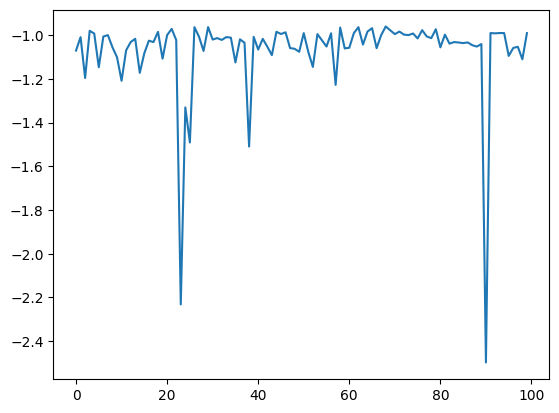
結果の確認
[6]:
plt.plot(res.fx[0:res.total_num_search])
[6]:
[<matplotlib.lines.Line2D at 0x1300a2460>]
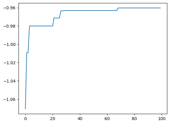
[7]:
best_fx, best_action = res.export_all_sequence_best_fx()
plt.plot(best_fx)
[7]:
[<matplotlib.lines.Line2D at 0x134af5460>]
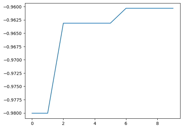
res.export_sequence_best_fx() により、各ステップまでに得られたベスト値とその action の履歴 を得られます。
res.export_all_sequence_best_fx() との違いは、simulator の評価毎ではなく、探索ステップ毎の情報になるという点です。(今回の場合は合計ステップ数は 10, 評価数は 100 です)
[8]:
best_fx, best_action = res.export_sequence_best_fx()
plt.plot(best_fx)
[8]:
[<matplotlib.lines.Line2D at 0x134b62df0>]