この jupyter notebook ファイルは ISSP Data Repository (v3.0.0 branch) から入手できます。

連続空間での最適化

ここまでのチュートリアルでは、特徴量空間を離散化してベイズ最適化を実行してきました。 PHYSBOは連続量のまま最適化することもできます。

連続空間で獲得関数を最大化するためのアルゴリズムとして、ランダムサーチが実装されています。 また、最適化ライブラリとして、ODAT-SEを使用することもできます。 これは pip を用いてインストール可能です。

python3 -m pip install odatse

基本的な使い方

まずは必要なモジュールをインポートします。

import numpy as np
import physbo
import matplotlib.pyplot as plt

Cythonized version of physbo is used

最適化したい関数 simulator について、離散版では候補点の番号 action を入力として受け取りましたが、連続版では座標 x を直接入力として受け取ります。 x は \(N\times D\) の配列で、\(N\) は計算するデータの数、\(D\) は特徴量の次元数です。

def simulator(x):
    return -np.sum(x**2, axis=1)

特徴量空間の下限と上限をそれぞれ min_X と max_X で指定します。

min_X = [-2.0, -2.0]
max_X = [2.0, 2.0]

連続空間版の Policy クラスは physbo.search.range.Policy です。 コンストラクタには min_X と max_X を指定します。 また、離散空間版と同様に mpi4py.MPI.Comm を comm として渡すことで並列実行が可能です。 set_seed メソッドを用いて乱数のシードを設定することもできます。

seed = 31415
policy = physbo.search.range.Policy(min_X=min_X, max_X=max_X)
policy.set_seed(seed)

一度 Policy クラスを作成してからは、離散空間版と同様の流れで最適化を実行できます。 まずは、サロゲートモデルを学習するための初期訓練データを作成するために、 random_search を実行します。

policy.random_search(max_num_probes=10, simulator=simulator)

0001-th step: f(x) = -0.831185 (action=[0.58327442 0.70069668])
   current best f(x) = -0.831185 (best action=[0.58327442 0.70069668])

0002-th step: f(x) = -5.914186 (action=[1.88281594 1.53921746])
   current best f(x) = -0.831185 (best action=[0.58327442 0.70069668])

0003-th step: f(x) = -4.352756 (action=[1.63626337 1.29437187])
   current best f(x) = -0.831185 (best action=[0.58327442 0.70069668])

0004-th step: f(x) = -0.237057 (action=[-0.05316112  0.48397432])
   current best f(x) = -0.237057 (best action=[-0.05316112  0.48397432])

0005-th step: f(x) = -0.488353 (action=[ 0.57404985 -0.39852174])
   current best f(x) = -0.237057 (best action=[-0.05316112  0.48397432])

0006-th step: f(x) = -2.441356 (action=[1.50087645 0.43442582])
   current best f(x) = -0.237057 (best action=[-0.05316112  0.48397432])

0007-th step: f(x) = -3.440784 (action=[-1.57320004 -0.98276443])
   current best f(x) = -0.237057 (best action=[-0.05316112  0.48397432])

0008-th step: f(x) = -3.452632 (action=[-1.85812001  0.00465691])
   current best f(x) = -0.237057 (best action=[-0.05316112  0.48397432])

0009-th step: f(x) = -0.764532 (action=[ 0.46977882 -0.73745485])
   current best f(x) = -0.237057 (best action=[-0.05316112  0.48397432])

0010-th step: f(x) = -1.850471 (action=[-0.63939092 -1.20068727])
   current best f(x) = -0.237057 (best action=[-0.05316112  0.48397432])

<physbo.search.range._history.History at 0x12afa6250>

次に、 bayes_search でベイズ最適化を実行します。

res = policy.bayes_search(max_num_probes=10, simulator=simulator, score="EI")

Start the initial hyper parameter searching ...
Done

Start the hyper parameter learning ...
0 -th epoch marginal likelihood 14.586042968393606
50 -th epoch marginal likelihood 14.234874815492592
100 -th epoch marginal likelihood 14.063504009485214
150 -th epoch marginal likelihood 13.916750623078872
200 -th epoch marginal likelihood 13.772691286779512
250 -th epoch marginal likelihood 13.633003306706115
300 -th epoch marginal likelihood 13.49920085405347
350 -th epoch marginal likelihood 13.371932369305052
400 -th epoch marginal likelihood 13.251396114620242
450 -th epoch marginal likelihood 13.13755169992651
500 -th epoch marginal likelihood 13.03022856247339
Done

0011-th step: f(x) = -5.026362 (action=[-1.03592362  1.98827161])
   current best f(x) = -0.237057 (best action=[-0.05316112  0.48397432])

0012-th step: f(x) = -0.028634 (action=[0.1327553  0.10492853])
   current best f(x) = -0.028634 (best action=[0.1327553  0.10492853])

0013-th step: f(x) = -0.013414 (action=[0.07031902 0.09202588])
   current best f(x) = -0.013414 (best action=[0.07031902 0.09202588])

0014-th step: f(x) = -0.057856 (action=[0.23418776 0.05488579])
   current best f(x) = -0.013414 (best action=[0.07031902 0.09202588])

0015-th step: f(x) = -0.012249 (action=[ 0.110677   -0.00028234])
   current best f(x) = -0.012249 (best action=[ 0.110677   -0.00028234])

0016-th step: f(x) = -0.015602 (action=[0.12295699 0.02198239])
   current best f(x) = -0.012249 (best action=[ 0.110677   -0.00028234])

0017-th step: f(x) = -0.026756 (action=[0.11124983 0.11991566])
   current best f(x) = -0.012249 (best action=[ 0.110677   -0.00028234])

0018-th step: f(x) = -0.025519 (action=[0.13646757 0.08304057])
   current best f(x) = -0.012249 (best action=[ 0.110677   -0.00028234])

0019-th step: f(x) = -0.005797 (action=[0.07576489 0.00754463])
   current best f(x) = -0.005797 (best action=[0.07576489 0.00754463])

0020-th step: f(x) = -0.032290 (action=[0.09645697 0.15161167])
   current best f(x) = -0.005797 (best action=[0.07576489 0.00754463])

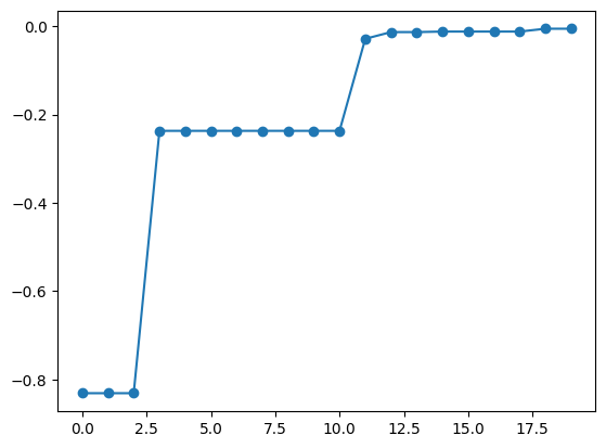
bayes_search 関数の返り値 res にはベイズ最適化の過程が保存されています。 export_sequence_best_fx メソッドを用いることで、各ステップでの最適化結果を取得できます。

best_fx, best_X = res.export_sequence_best_fx()

plt.plot(best_fx, "o-")

[<matplotlib.lines.Line2D at 0x12b0735b0>]

獲得関数の最適化アルゴリズム

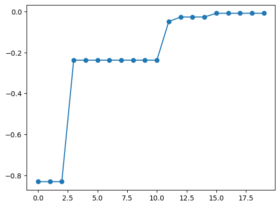
獲得関数の最適化として、デフォルトではランダムサーチが行われます。つまり、 nsamples = 1000 個の候補点をランダムに選び、その中で最も獲得関数が大きい点を選びます。 nsamples の値を変更する場合には、 physbo.search.optimizer.random.Optimizer を用います。 例えば、 nsamples = 100 にしたい場合は、次のように random_optimizer を作成し、 bayes_search 関数の optimizer キーワードに渡します。

random_optimizer = physbo.search.optimize.random.Optimizer(min_X=min_X, max_X=max_X, nsamples=100)

policy = physbo.search.range.Policy(min_X=min_X, max_X=max_X)
policy.set_seed(seed)
policy.random_search(max_num_probes=10, simulator=simulator)

res = policy.bayes_search(max_num_probes=10, simulator=simulator, score="EI", optimizer=random_optimizer)

best_fx, best_X = res.export_sequence_best_fx()

plt.plot(best_fx, "o-")

0001-th step: f(x) = -0.831185 (action=[0.58327442 0.70069668])
   current best f(x) = -0.831185 (best action=[0.58327442 0.70069668])

0002-th step: f(x) = -5.914186 (action=[1.88281594 1.53921746])
   current best f(x) = -0.831185 (best action=[0.58327442 0.70069668])

0003-th step: f(x) = -4.352756 (action=[1.63626337 1.29437187])
   current best f(x) = -0.831185 (best action=[0.58327442 0.70069668])

0004-th step: f(x) = -0.237057 (action=[-0.05316112  0.48397432])
   current best f(x) = -0.237057 (best action=[-0.05316112  0.48397432])

0005-th step: f(x) = -0.488353 (action=[ 0.57404985 -0.39852174])
   current best f(x) = -0.237057 (best action=[-0.05316112  0.48397432])

0006-th step: f(x) = -2.441356 (action=[1.50087645 0.43442582])
   current best f(x) = -0.237057 (best action=[-0.05316112  0.48397432])

0007-th step: f(x) = -3.440784 (action=[-1.57320004 -0.98276443])
   current best f(x) = -0.237057 (best action=[-0.05316112  0.48397432])

0008-th step: f(x) = -3.452632 (action=[-1.85812001  0.00465691])
   current best f(x) = -0.237057 (best action=[-0.05316112  0.48397432])

0009-th step: f(x) = -0.764532 (action=[ 0.46977882 -0.73745485])
   current best f(x) = -0.237057 (best action=[-0.05316112  0.48397432])

0010-th step: f(x) = -1.850471 (action=[-0.63939092 -1.20068727])
   current best f(x) = -0.237057 (best action=[-0.05316112  0.48397432])

Start the initial hyper parameter searching ...
Done

Start the hyper parameter learning ...
0 -th epoch marginal likelihood 14.586042968393606
50 -th epoch marginal likelihood 14.234874815492592
100 -th epoch marginal likelihood 14.063504009485214
150 -th epoch marginal likelihood 13.916750623078872
200 -th epoch marginal likelihood 13.772691286779512
250 -th epoch marginal likelihood 13.633003306706115
300 -th epoch marginal likelihood 13.49920085405347
350 -th epoch marginal likelihood 13.371932369305052
400 -th epoch marginal likelihood 13.251396114620242
450 -th epoch marginal likelihood 13.13755169992651
500 -th epoch marginal likelihood 13.03022856247339
Done

0011-th step: f(x) = -3.969688 (action=[-0.55371092  1.91392061])
   current best f(x) = -0.237057 (best action=[-0.05316112  0.48397432])

0012-th step: f(x) = -0.048301 (action=[ 0.09981879 -0.19579904])
   current best f(x) = -0.048301 (best action=[ 0.09981879 -0.19579904])

0013-th step: f(x) = -0.026065 (action=[0.00582793 0.16134044])
   current best f(x) = -0.026065 (best action=[0.00582793 0.16134044])

0014-th step: f(x) = -0.029637 (action=[-0.03315978  0.16893146])
   current best f(x) = -0.026065 (best action=[0.00582793 0.16134044])

0015-th step: f(x) = -6.287502 (action=[ 1.84812961 -1.69467382])
   current best f(x) = -0.026065 (best action=[0.00582793 0.16134044])

0016-th step: f(x) = -0.007927 (action=[ 0.06895685 -0.05632176])
   current best f(x) = -0.007927 (best action=[ 0.06895685 -0.05632176])

0017-th step: f(x) = -0.011240 (action=[0.10157691 0.03036993])
   current best f(x) = -0.007927 (best action=[ 0.06895685 -0.05632176])

0018-th step: f(x) = -0.060419 (action=[ 0.1940892  -0.15082425])
   current best f(x) = -0.007927 (best action=[ 0.06895685 -0.05632176])

0019-th step: f(x) = -0.016852 (action=[-0.12738362  0.02501082])
   current best f(x) = -0.007927 (best action=[ 0.06895685 -0.05632176])

0020-th step: f(x) = -0.093609 (action=[0.12668816 0.27849452])
   current best f(x) = -0.007927 (best action=[ 0.06895685 -0.05632176])

[<matplotlib.lines.Line2D at 0x12b167a60>]

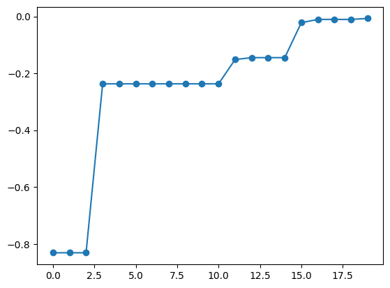
physbo.search.optimize.random.Optimizer 以外のオプティマイザを使うことで、ランダムサーチ以外の最大化アルゴリズムを利用できます。 PHYSBOでは、ODAT-SEを用いるオプティマイザ physbo.search.optimize.odatse.Optimizer を提供しています。このライブラリは

• 「exchange」: レプリカ交換モンテカルロ法

• 「pamc」: ポピュレーションアニーリングモンテカルロ法

• 「minsearch」: Nelder-Mead法

• 「mapper」: グリッドサーチ

• 「bayes」: ベイズ最適化

の5つのアルゴリズムを用いて最適化問題を解くことができます。 ODAT-SEのアルゴリズムやハイパーパラメータは、ODAT-SEの入力ファイルの [algorithm] セクションに相当する辞書を用いて指定します。

physbo.search.optimize.odatse.default_alg_dict 関数でこの辞書の雛形ができるので、必要に応じてパラメータを修正します。

import physbo.search.optimize.odatse
odatse_alg_dict = physbo.search.optimize.odatse.default_alg_dict(min_X=min_X,
                                                                 max_X=max_X,
                                                                 algorithm_name="exchange")

# show the default parameters for the exchange algorithm
odatse_alg_dict

{'name': 'exchange',
 'seed': 12345,
 'param': {'min_list': array([-2., -2.]),
  'max_list': array([2., 2.]),
  'step_list': array([0.04, 0.04])},
 'exchange': {'numsteps': 1000,
  'numsteps_exchange': 10,
  'Tmin': 0.1,
  'Tmax': 10.0,
  'Tlogspace': True,
  'nreplica_per_proc': 10}}

odatse_alg_dict を physbo.search.optimize.odatse.Optimizer に渡してオプティマイザ odatse_optimizer を作成します。 これを random_optimizer と同様に bayes_search 関数の optimizer キーワードに渡すことで、ODAT-SEを用いた最適化を行えます。

odatse_optimizer = physbo.search.optimize.odatse.Optimizer(alg_dict=odatse_alg_dict)

policy = physbo.search.range.Policy(min_X=min_X, max_X=max_X)
policy.set_seed(seed)
policy.random_search(max_num_probes=10, simulator=simulator)

res = policy.bayes_search(max_num_probes=10,
                          simulator=simulator,
                          optimizer=odatse_optimizer,
                          score="EI")

best_fx, best_X = res.export_sequence_best_fx()

plt.plot(best_fx, "o-")

[<matplotlib.lines.Line2D at 0x13a953130>]